bicortex

Amazon Redshift Review – Data Warehouse in the Cloud Is Here, Part 2

Background And Environment Specs Recap

In the FIRST part of this series I briefly explored the background of Amazon’s Redshift data warehouse offering as well as outlined the environments and tools used for managing test datasets. I also recreated TICKIT database schema on all instances provisioned for testing and preloaded them with dummy data. In this post I would like to explore the performance findings from running a bunch of sample SQL queries to find out how they behave under load. Final post outlining how to connect and use data stored in Redshift can be found HERE.

As mentioned in my FIRST post, all datasets which populated TICKIT sample database were quite small so I needed to synthetically expand one of the tables in order to increase data volumes to make the whole exercise viable. Using nothing but SQL I ‘stretched out’ my Sales fact table to around 50,000,000 records which is hardly enough for any database to break a sweat, but given the free storage limit on Amazon S3 is only 5 GB (you can also use DynamoDB as a file storage) and that my home internet bandwidth is still stuck on ADSL2 I had to get a little creative with the SQL queries rather than try to push for higher data volumes. Testing methodology was quite simple here – using mocked-up SQL SELECT statements, for each query executed I recorded execution time on all environments and plucked them into a graph for comparison. None of those statements represent any business function so I did not focus on any specific output or result; the idea was to simply make them run and wait until completion, taking note of how long it took from beginning to end. Each time the query was executed, the instance got restarted to ensure cold cache and full system resources available to database engine. I also tried to make my SQL as generic as possible. By default, SQL is not a very verbose language, with a not a lot of dichotomies between different vendors. Most of the core syntax principles apply to both PG/SQL and Microsoft T-SQL alike. However, there are some small distinctions which can get ‘lost in translation’ therefore I tried to keep the queries are as generic and universal as possible.

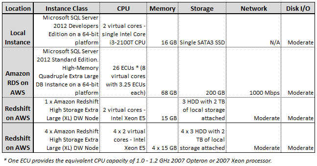
As far as physical infrastructure composition, the image below contains a quick recap of the testing environment used for this evaluation. Initially, I planned to test my queries on 3 different Redshift deployments – a single and a multi-node Redshift XL instance as well as a single Redshift 8XL instance, however, after casually running a few queries and seeing the performance level Redshift is capable of I decided to scale back and run only with Redshift XL class in a single and multi-node configurations.

Graphing the results, for simplicity sake, I assigned the following monikers to each environment:

• ‘Local Instance’ – my local SQL Server 2012 deployment
• ‘RDS SQL Server’ – High-Memory Quadruple Extra Large DB Instance of SQL Server 2012
• ‘1 x Redshift XL’ – Single High Storage Extra Large (XL) Redshift DW node (1 x dw.hs1.xlarge)
• ‘4 x Redshift XL’ – Four High Storage Extra Large (XL) Redshift DW nodes (4 x dw.hs1.xlarge)

Test Results

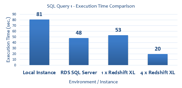
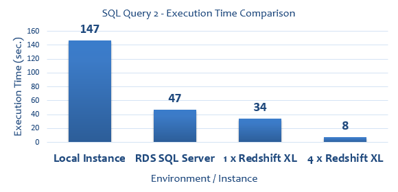
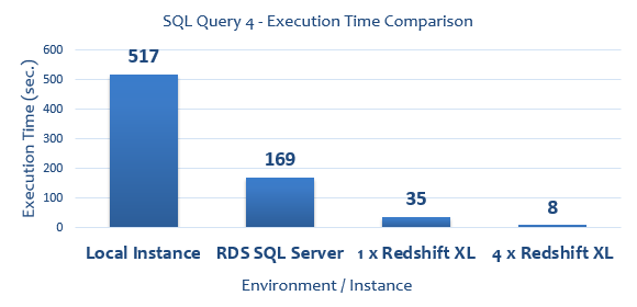
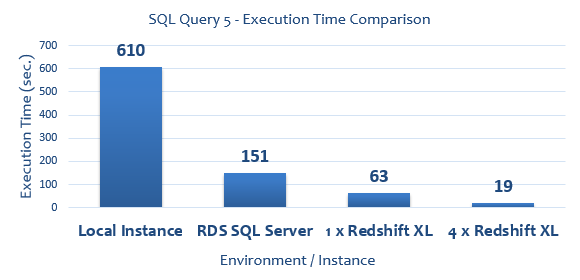
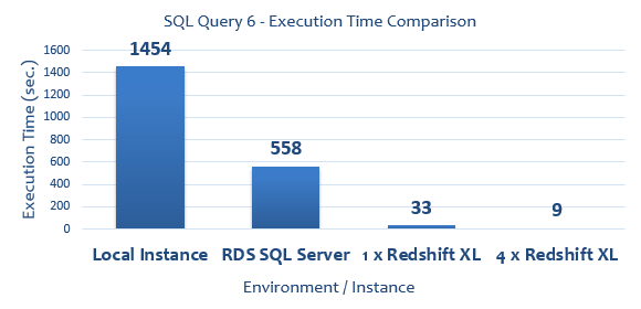
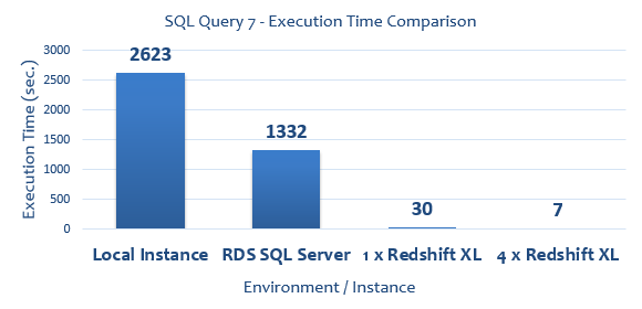
All SQL queries run to collect execution times (expressed in seconds) as well as graphical representation of their duration are as per below.

--QUERY 1
SELECT COUNT(*) FROM
	(SELECT COUNT(*) AS counts, salesid, listid, sellerid, buyerid,
	eventid, dateid, qtysold, pricepaid, commission, saletime
	FROM sales
	GROUP BY salesid, listid, sellerid, buyerid, eventid,
	dateid, qtysold, pricepaid, commission, saletime) sub

--QUERY 2
WITH cte AS (
	SELECT
		SUM(s.pricepaid) AS pricepaid,
		sub.*,
		u1.email,
		DENSE_RANK() OVER (PARTITION BY sub.totalprice ORDER BY d.caldate DESC) AS daterank
	FROM sales s  JOIN
		(SELECT l.totalprice, l.listid, v.venuecity, c.catdesc
		FROM listing l
		LEFT JOIN event e on l.eventid = e.eventid
		INNER JOIN category c on e.catid = c.catid
		INNER JOIN venue v on e.venueid = v.venueid
		GROUP BY v.venuecity, c.catdesc, l.listid, l.totalprice) sub
	ON s.listid = sub.listid
	LEFT JOIN users u1 on s.buyerid = u1.userid
	LEFT JOIN Date d on d.dateid = s.dateid
	GROUP BY sub.totalprice, sub.listid, sub.venuecity, sub.catdesc, u1.email, d.caldate)
SELECT COUNT(*) FROM cte

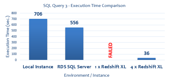
--QUERY 3
SELECT COUNT(*) FROM(
SELECT s.*, u.* FROM sales s
		LEFT JOIN event e on s.eventid = e.eventid
		LEFT JOIN date d on d.dateid = s.dateid
		LEFT JOIN users u on u.userid = s.buyerid
		LEFT JOIN listing l on l.listid = s.listid
		LEFT JOIN category c on c.catid = e.catid
		LEFT JOIN venue v on v.venueid = e.venueid
	INTERSECT
SELECT s.*, u.* FROM sales s
		LEFT JOIN event e on s.eventid = e.eventid
		LEFT JOIN date d on d.dateid = s.dateid
		LEFT JOIN users u on u.userid = s.buyerid
		LEFT JOIN listing l on l.listid = s.listid
		LEFT JOIN category c on c.catid = e.catid
		LEFT JOIN venue v on v.venueid = e.venueid
		WHERE d.holiday =0) sub

--QUERY 4
WITH Temp (eventname, starttime, eventid) AS
	(SELECT ev.eventname, ev.starttime, ev.eventid
	FROM Event ev
	WHERE	NOT EXISTS	
			(SELECT 1 FROM Sales s
			WHERE s.pricepaid  > 500 AND s.pricepaid < 900 AND s.eventid = ev.eventid) 	
			AND  EXISTS	(SELECT 1 FROM Sales s 
			WHERE s.qtysold  >= 4 AND s.eventid = ev.eventid))
SELECT COUNT(t.eventid) AS EvCount,
SUM(l.totalprice)  - SUM((CAST(l.numtickets AS Decimal(8,2)) * l.priceperticket * 0.9)) as TaxPaid
FROM Temp t JOIN Listing l ON l.eventid = t.eventid
WHERE t.starttime <= l.listtime

--QUERY 5
SELECT COUNT(*) FROM
	(SELECT
		SUM(sub1.pricepaid) AS price_paid,
		sub1.caldate AS date,
		sub1.username
	FROM
		(select  s.pricepaid, d.caldate, u.username
		FROM Sales s
		LEFT JOIN date d on s.dateid=s.dateid
		LEFT JOIN users u on s.buyerid = u.userid
		WHERE s.saletime BETWEEN '2008-12-01' AND '2008-12-31'
		) sub1
	GROUP BY sub1.caldate, sub1.username
	) as sub2

--QUERY 6
WITH CTE1 (c1) AS
		(SELECT COUNT(1) as c1 FROM Sales s
		WHERE saletime BETWEEN '2008-12-01' AND '2008-12-31' 
		GROUP BY salesid 
		HAVING COUNT(*)=1),
	CTE2 (c2) AS
		(SELECT COUNT(1) as c2 FROM Listing e
		WHERE listtime BETWEEN '2008-12-01' AND '2008-12-31' 
		GROUP BY listid	
		HAVING COUNT(*)=1),
	CTE3 (c3) AS
		(SELECT COUNT(1) as c3 FROM Date d	
		GROUP BY dateid 
		HAVING COUNT(*)=1)
SELECT COUNT(*) FROM Cte1
					RIGHT JOIN CTE2 ON CTE1.c1 <> CTE2.c2
					RIGHT JOIN CTE3 ON CTE3.c3 = CTE2.c2 and CTE3.c3 <> CTE1.c1
					GROUP BY CTE1.c1
					HAVING COUNT(*)>1

--QUERY 7
SELECT COUNT(*) FROM
(SELECT COUNT(*) as c FROM sales s
WHERE s.saletime BETWEEN '2008-12-01' AND '2008-12-31'
GROUP BY salesid
HAVING COUNT(*)=1) a
LEFT JOIN
(SELECT COUNT(*) as c FROM date d
WHERE d.week = 1
GROUP BY dateid
HAVING COUNT(*)=1) b
ON a.c <> b.c
LEFT JOIN
(SELECT COUNT(*) as c FROM listing l
WHERE l.listtime BETWEEN '2008-12-01' AND '2008-12-31'
GROUP BY listid
HAVING COUNT(*)=1) c
ON a.c <> c.c AND b.c <> c.c
LEFT JOIN
(SELECT COUNT(*) as c FROM venue v
GROUP BY venueid
HAVING COUNT(*)=1) d
ON a.c <> d.c AND b.c <> d.c AND c.c <> d.c

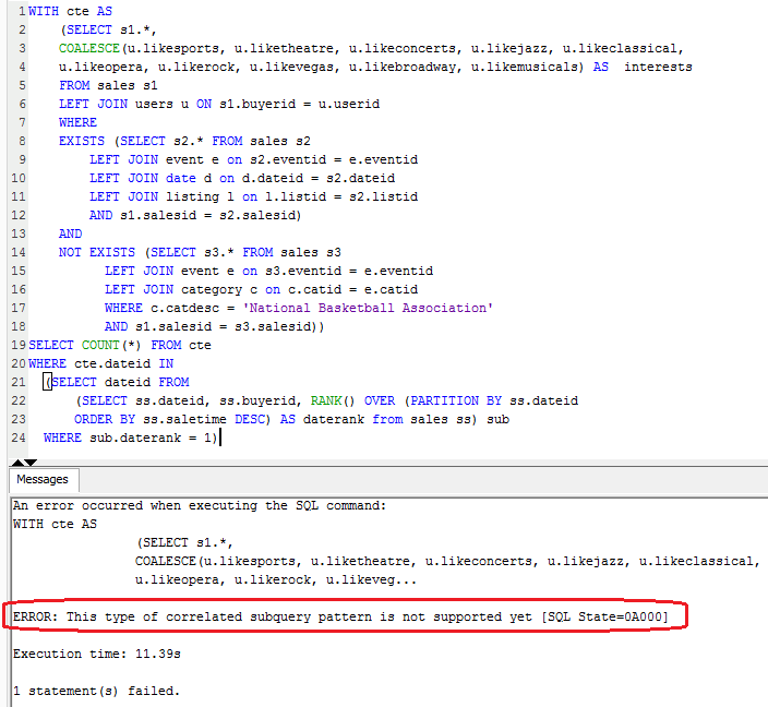
Finally, before diving into conclusion section, a short mention of a few unexpected hiccups along the way. On a single node deployment 2 queries failed for two different reasons. First one returned an error message stating that ‘This type of correlated subquery pattern is not supported yet’ (see image below).

Because of this, I decided to remove this query from the overall results tally leaving me with 7 SQL statements for testing. Query 3 on the other hand failed with ‘Out of memory’ message on the client side and another cryptic error showing up in management console as per images below (click on image to enlarge).

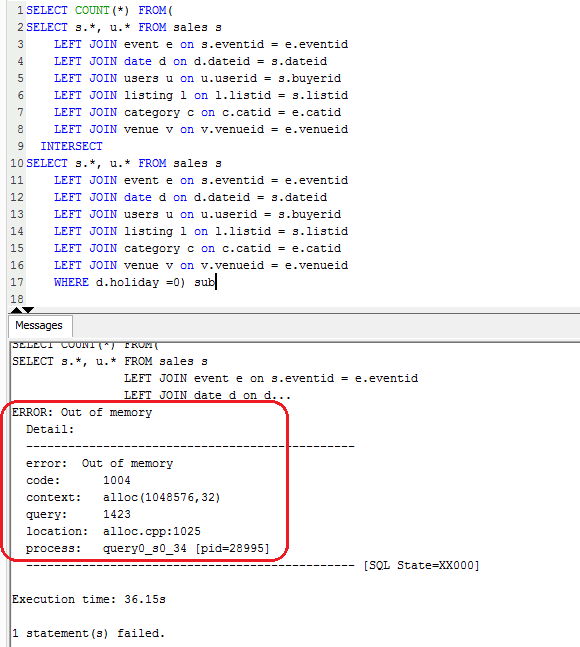
I think that inadequate memory allocation issue was due to the lack of resources provisioned as it only appeared when running on a single node – the multi-node deployment executed without issues. Nevertheless, it was disappointing to see Redshift not coping very well with memory allocation and management, especially given that same query run fine (albeit slow) on both of the SQL Server databases.

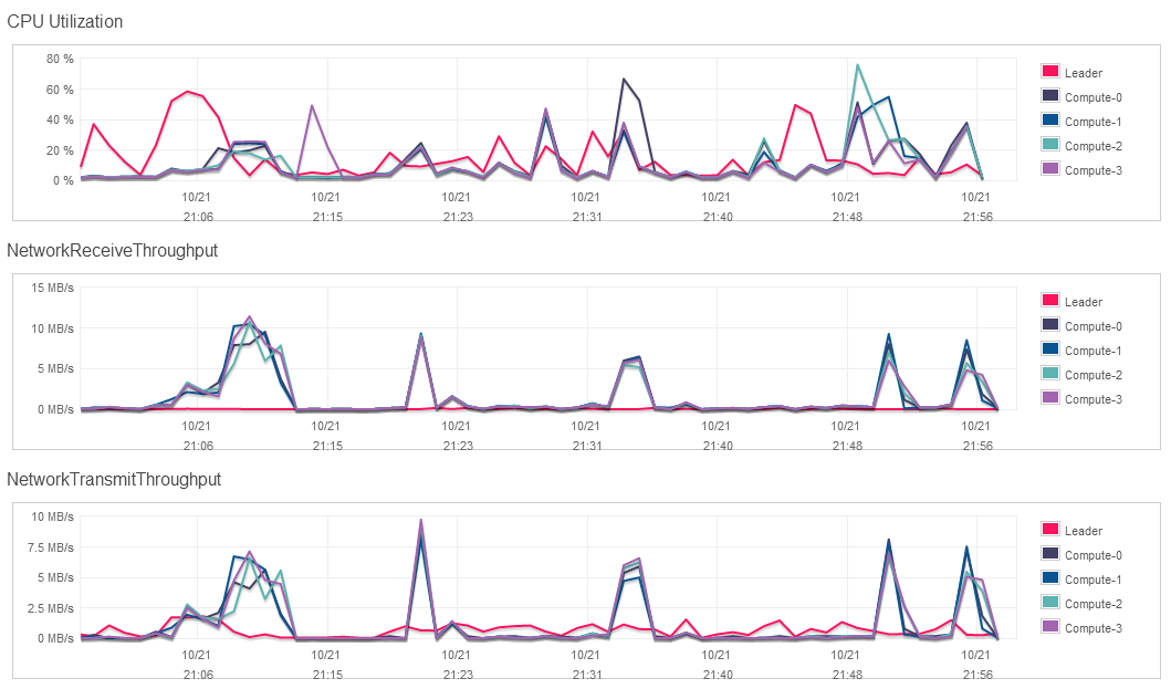
For reference, below is a resource consumption graph (3 parameters included) for the multi-node deployment of Amazon Redshift during queries execution.

Performance Verdict

I don’t think I have to interpret the results in much detail here – they are pretty much self-explanatory. Redshift, with the exception of few quibbles where SQL query was either unsupported or too much to handle for its default memory management, completely outrun the opposition. As I already stated in PART 1 of this series, relational database setup is probably not the best option for reading vast volumes of data with heavy aggregations thrown into the mix (that’s what SSAS is for when using Microsoft as a vendor) but at the same time I never expected such blazing performance (per dollar) from the Amazon offering. At this point I wish I had more data to throw at it as 50,000,000 records in my largest table is not really MPP database playground but nevertheless, Redshift screamed through what a gutsy SQL Server RDS deployment costing more completely chocked on. Quite impressive, although having heard other people’s comments and opinions, some even going as far as saying that Redshift is a great alternative to Hadoop (providing data being structured and homogeneous), I was not surprised.

In the next part to this series – PART 3 – I will be looking at connecting to Redshift database using some popular reporting/data visualization tools e.g. Tableau too see if this technology makes it a viable backend solution not just for data storage but also for querying through third-party applications.

http://scuttle.org/bookmarks.php/pass?action=add

Posted in: Cloud Computing

Tags: Amazon Redshift, Big Data, Cloud Computing, MPP RDBMS, SQL Server

This entry was posted on Friday, November 1st, 2013 at 12:27 pm and is filed under Cloud Computing. You can follow any responses to this entry through the RSS 2.0 feed. You can leave a response, or trackback from your own site.