October 7th, 2013 / No Comments » / by admin
In two of my previous posts (HERE and HERE) I explored the concept of dynamic data synchronisation between tables in two different databases. Lately, I have been working with a client who required not only data to be replicated between individual tables but also the objects themselves. Data synchronisation can be easily achieved through embedded SSIS functionality or if dynamic configuration is required through THIS solution implementation, however, in this particular instance, the caveat laid with not just data but also with schema acquisition dynamisms – the client had no way of knowing what objects (names, types, definitions, data etc.) were added to the source database that required to be recreated on the target. Simply put it – all tables and their data as well as stored procedures, functions and views had to be recreated on a daily/nightly basis in the destination database without going through the exercise of selecting or nominating them individually, which SSIS is more than capable of performing through Transfer SQL Server Objects Task.
In order to demonstrate how this functionality is resolved, let’s first create a sandbox environment with two databases and a bunch of dummy objects. Source_DB is the database where stored procedure, function, view and a few tables will be placed on, whereas Target_DB, as the name implies, will become our destination database, not containing any user defined objects just yet.
USE [master]
GO
IF EXISTS (SELECT name FROM sys.databases WHERE name = N'Source_DB')
BEGIN
-- Close connections to the DW_Sample database
ALTER DATABASE [Source_DB] SET SINGLE_USER WITH ROLLBACK IMMEDIATE
DROP DATABASE [Source_DB]
END
GO
CREATE DATABASE [Source_DB]

IF EXISTS (SELECT name FROM sys.databases WHERE name = N'Target_DB')
BEGIN
-- Close connections to the DW_Sample database
ALTER DATABASE [Target_DB] SET SINGLE_USER WITH ROLLBACK IMMEDIATE
DROP DATABASE [Target_DB]
END
GO
CREATE DATABASE [Target_DB]

USE Source_DB
CREATE TABLE Tbl1 (
ID int NOT NULL,
Sample_Data_Col1 varchar (50) NOT NULL,
Sample_Data_Col2 varchar (50) NOT NULL,
Sample_Data_Col3 varchar (50) NOT NULL)
GO

USE Source_DB
DECLARE @rowcount int = 0
WHILE @rowcount < 10000
	BEGIN
		SET NOCOUNT ON
		INSERT INTO Tbl1
		(ID, Sample_Data_Col1, Sample_Data_Col2, Sample_Data_Col3)
		SELECT
		@rowcount,
		'Sample_Data' + CAST(@rowcount as varchar(10)),
		'Sample_Data' + CAST(@rowcount as varchar(10)),
		'Sample_Data' + CAST(@rowcount as varchar(10))
		SET @rowcount = @rowcount + 1
	END
GO

SELECT * INTO Tbl2 FROM Tbl1
SELECT * INTO Tbl3 FROM Tbl1
SELECT * INTO Tbl4 FROM Tbl1
SELECT * INTO Tbl5 FROM Tbl1
GO

CREATE PROCEDURE sp_SampleProcedure1
AS
BEGIN
	SET NOCOUNT ON;
	SELECT GetDate()
END
GO

CREATE FUNCTION dbo.ufn_SampleFunction1 (@ID int)
RETURNS TABLE
AS
RETURN
(SELECT * FROM Tbl1 WHERE ID = @ID)
GO

CREATE VIEW vw_SampleTop10
AS
SELECT TOP (10) * FROM dbo.Tbl1
Once the code executed, we are ready to create our objects synchronisation stored procedure which should account for all user defined objects and recreate them on the destination database – these will include tables with their corresponding data, functions, views and additional stored procedures and can be modified to encompass other types as per additional requirements. The code simply queries a collection of system objects to fetch their names and definitions, builds a temporary table to store this metadata and finally using cursors replicates those on a target database.
USE [target_DB]
IF EXISTS (SELECT * FROM sys.objects WHERE object_id = OBJECT_ID(N'[dbo].[usp_SyncDBObjects]')
AND type IN (N'P',N'PC'))
DROP PROCEDURE [dbo].[usp_SyncDBObjects]
GO

CREATE PROCEDURE [usp_SyncDBObjects]
@SourceDBName       varchar (256),
@SourceSchemaName   varchar (50),
@TargetDBName       varchar (256),
@TargetSchemaName   varchar (50)
AS
BEGIN

    SET NOCOUNT ON
    DECLARE @Err_Msg varchar (max)
    DECLARE @IsDebugMode bit = 0
    DECLARE @SQLSource nvarchar (max) =
    'INSERT INTO #TempTbl
    (ObjectID, ObjectName, SchemaName, DBName, ObjectType, ObjectDefinition)
    SELECT DISTINCT
    o.object_id,o.name, '''+@SourceSchemaName+''', '''+@SourceDBName+''',''Table'',''N/A''
    FROM   '+@SourceDBName+'.sys.tables t
    JOIN '+@SourceDBName+'.sys.schemas s ON t.schema_id = s.schema_id
    JOIN '+@SourceDBName+'.sys.objects o ON t.schema_id = o.schema_id
    WHERE S.name = '''+@SourceSchemaName+''' and o.type = ''U''
    UNION ALL
    SELECT DISTINCT
    o.object_id, o.name, '''+@SourceSchemaName+''', '''+@SourceDBName+''',''View'', m.definition
    FROM   '+@SourceDBName+'.sys.tables t
    JOIN '+@SourceDBName+'.sys.schemas s ON t.schema_id = s.schema_id
    JOIN '+@SourceDBName+'.sys.objects o ON t.schema_id = o.schema_id
    LEFT JOIN '+@SourceDBName+'.sys.sql_modules m ON m.object_id = o.object_id
    WHERE S.name = '''+@SourceSchemaName+''' and o.type = ''V''
    UNION ALL
    SELECT DISTINCT
    o.object_id, o.name, '''+@SourceSchemaName+''', '''+@SourceDBName+''',''Stored Procedure'', m.definition
    FROM   '+@SourceDBName+'.sys.tables t
    JOIN '+@SourceDBName+'.sys.schemas s ON t.schema_id = s.schema_id
    JOIN '+@SourceDBName+'.sys.objects o ON t.schema_id = o.schema_id
    LEFT JOIN '+@SourceDBName+'.sys.sql_modules m ON m.object_id = o.object_id
    WHERE S.name = '''+@SourceSchemaName+''' and o.type = ''P''
    UNION ALL
    SELECT DISTINCT
    o.object_id, o.name, '''+@SourceSchemaName+''', '''+@SourceDBName+''',''Function'', m.definition
    FROM   '+@SourceDBName+'.sys.tables t
    JOIN '+@SourceDBName+'.sys.schemas s ON t.schema_id = s.schema_id
    JOIN '+@SourceDBName+'.sys.objects o ON t.schema_id = o.schema_id
    LEFT JOIN '+@SourceDBName+'.sys.sql_modules m ON m.object_id = o.object_id
    WHERE S.name = '''+@SourceSchemaName+''' and o.type IN (''TF'',''IF'', ''FN'', ''FS'')'

    IF OBJECT_ID('tempdb..#TempTbl') IS NOT NULL
    DROP TABLE #TempTbl

    CREATE TABLE #TempTbl
    (ID int IDENTITY (1,1),
    ObjectID            int,
    ObjectName          varchar (256),
    SchemaName          varchar (50),
    DBName              varchar (50),
    ObjectType          varchar (20),
    ObjectDefinition    varchar (max))

    EXEC sp_executesql @SQLSource

    IF NOT EXISTS (SELECT 1 FROM #TempTbl a WHERE a.dbname = @SourceDBName and a.SchemaName = @SourceSchemaName)
    BEGIN
        SET
        @Err_Msg = 'Source database objects cannot be fetched. You nominated ''['+@SourceDBName+']'' database on a ''['+@SourceSchemaName+']'' schema. '
        RAISERROR (
        @Err_Msg  -- Message text.
        ,16 -- Severity.
            ,1 -- State.
                    )
        RETURN
    END

    IF @IsDebugMode = 1
    SELECT * FROM #TempTbl
    --IF @IsDebugMode = 1
        PRINT ''
        PRINT 'The following objects based on Source vs Target comparison will be synchronised between ''['+@TargetDBName+']'' and ''['+@SourceDBName+']''...'
        DECLARE @ID int
        DECLARE @TblName varchar (256)
        DECLARE cur CURSOR FOR
            SELECT ID, ObjectName FROM #TempTbl
            OPEN cur
            FETCH NEXT FROM cur INTO @ID, @TblName
            WHILE @@FETCH_STATUS = 0
            BEGIN
                PRINT '' + CAST(@ID as varchar (20))+'. '+ @TblName +''
                FETCH NEXT FROM cur INTO @ID, @TblName
            END
        CLOSE cur
        DEALLOCATE cur
    DECLARE @ObjectName varchar (256)
    DECLARE @sql_select varchar (max)
    DECLARE @sql_drop varchar (max)
    DECLARE @sql_definition varchar (max)
	DECLARE @Err int
    PRINT ''
    PRINT 'Starting objects synchronisation process...'
    PRINT ''
    PRINT 'Recreating tables and data...'

    DECLARE db_cursor CURSOR FORWARD_ONLY
        FOR
            SELECT ObjectName
            FROM #TempTbl t
            WHERE t.ObjectType = 'table'
            OPEN db_cursor
			SELECT @Err = @@Error IF @Err <> 0 BEGIN DEALLOCATE db_cursor RETURN @Err END
            FETCH NEXT
            FROM db_cursor INTO @ObjectName
                WHILE @@FETCH_STATUS = 0
                    BEGIN
						BEGIN TRY
							BEGIN TRANSACTION
                            PRINT 'DROPPING TABLE '+@TargetDBName+'.'+@TargetSchemaName+'.'+@ObjectName+''
                            SET @SQL_drop       =   'IF EXISTS (SELECT * FROM '+@TargetDBName+'.INFORMATION_SCHEMA.TABLES WHERE TABLE_NAME
                                                = '''+@ObjectName+''') DROP TABLE '+@TargetDBName+'.'+@TargetSchemaName+'.'+@ObjectName+''
                            EXEC sp_sqlexec @SQL_drop
							COMMIT TRANSACTION
						END TRY
						BEGIN CATCH
							ROLLBACK TRANSACTION
							SELECT
							 ERROR_NUMBER       () AS ErrorNumber
							,ERROR_SEVERITY     () AS ErrorSeverity
							,ERROR_STATE        () AS ErrorState
							,ERROR_PROCEDURE    () AS ErrorProcedure
							,ERROR_LINE         () AS ErrorLine
							,ERROR_MESSAGE      () AS ErrorMessage;
						END CATCH

						BEGIN TRY
							BEGIN TRANSACTION
							PRINT 'SELECTING INTO ' + @SourceDBName + '.' + @SourceSchemaName + '.' + @ObjectName + ' FROM '+ @TargetDBName + '.' + @TargetSchemaName + '.' + @ObjectName + ''
                            SET @SQL_select     =   'SELECT * INTO '+@TargetDBName+'.'+@TargetSchemaName+'.'+@ObjectName+'
                                                FROM '+@SourceDBName+'.'+@SourceSchemaName+'.'+@ObjectName+''
                            EXEC sp_sqlexec @SQL_select
							COMMIT TRANSACTION
						END TRY
						BEGIN CATCH
							ROLLBACK TRANSACTION
							SELECT
							 ERROR_NUMBER       () AS ErrorNumber
							,ERROR_SEVERITY     () AS ErrorSeverity
							,ERROR_STATE        () AS ErrorState
							,ERROR_PROCEDURE    () AS ErrorProcedure
							,ERROR_LINE         () AS ErrorLine
							,ERROR_MESSAGE      () AS ErrorMessage;
						END CATCH
                    FETCH NEXT FROM db_cursor INTO @ObjectName
                END
            CLOSE db_cursor
            DEALLOCATE db_cursor
    PRINT ''
    PRINT 'Recreating views...'
    DECLARE db_cursor CURSOR FORWARD_ONLY
        FOR
            SELECT ObjectName
            FROM #TempTbl t
            WHERE t.ObjectType = 'view'
            OPEN db_cursor
			SELECT @Err = @@Error IF @Err <> 0 BEGIN DEALLOCATE db_cursor RETURN @Err END
            FETCH NEXT
            FROM db_cursor INTO @ObjectName
                WHILE @@FETCH_STATUS = 0
					BEGIN
						BEGIN TRY
							BEGIN TRANSACTION
                            PRINT 'DROPPING VIEW '+@TargetDBName+'.'+@TargetSchemaName+'.'+@ObjectName+''
                            SET @SQL_drop       =   'IF EXISTS (SELECT * FROM '+@TargetDBName+'.INFORMATION_SCHEMA.TABLES WHERE TABLE_NAME
                                                = '''+@ObjectName+''') DROP VIEW '+@TargetSchemaName+'.'+@ObjectName+''
                            EXEC sp_sqlexec @SQL_drop
							COMMIT TRANSACTION
						END TRY
						BEGIN CATCH
							ROLLBACK TRANSACTION
							SELECT
							 ERROR_NUMBER       () AS ErrorNumber
							,ERROR_SEVERITY     () AS ErrorSeverity
							,ERROR_STATE        () AS ErrorState
							,ERROR_PROCEDURE    () AS ErrorProcedure
							,ERROR_LINE         () AS ErrorLine
							,ERROR_MESSAGE      () AS ErrorMessage;
						END CATCH

						BEGIN TRY
							BEGIN TRANSACTION
							PRINT 'CREATING VIEW ' + @ObjectName + ' on '+@TargetDBName+' from '+ @SourceDBName + '.' + @SourceSchemaName + '.' + @ObjectName + ' view'
							SET @SQL_select     =   (SELECT ObjectDefinition FROM #TempTbl WHERE ObjectName = @ObjectName)
                            EXEC sp_sqlexec @SQL_select
							COMMIT TRANSACTION
						END TRY
						BEGIN CATCH
							ROLLBACK TRANSACTION
							SELECT
							 ERROR_NUMBER       () AS ErrorNumber
							,ERROR_SEVERITY     () AS ErrorSeverity
							,ERROR_STATE        () AS ErrorState
							,ERROR_PROCEDURE    () AS ErrorProcedure
							,ERROR_LINE         () AS ErrorLine
							,ERROR_MESSAGE      () AS ErrorMessage;
						END CATCH
                    FETCH NEXT FROM db_cursor INTO @ObjectName
                END
            CLOSE db_cursor
            DEALLOCATE db_cursor
    PRINT ''
    PRINT 'Recreating functions...'
    DECLARE db_cursor CURSOR FORWARD_ONLY
        FOR
            SELECT ObjectName
            FROM #TempTbl t
            WHERE t.ObjectType = 'Function'
            OPEN db_cursor
			SELECT @Err = @@Error IF @Err <> 0 BEGIN DEALLOCATE db_cursor RETURN @Err END
            FETCH NEXT
            FROM db_cursor INTO @ObjectName
                WHILE @@FETCH_STATUS = 0
                    BEGIN
						BEGIN TRY
							BEGIN TRANSACTION
                            PRINT 'DROPPING FUNCTION '+@TargetDBName+'.'+@TargetSchemaName+'.'+@ObjectName+''
                            SET @SQL_drop       =   'IF EXISTS (SELECT * FROM '+@TargetDBName+'.'+@TargetSchemaName+'.sysobjects WHERE id = object_id('''+@ObjectName+''')
                                                    AND xtype IN (''TF'',''IF'', ''FN'', ''FS''))  DROP FUNCTION '+@TargetSchemaName+'.'+@ObjectName+''
                            EXEC sp_sqlexec @SQL_drop
							COMMIT TRANSACTION
						END TRY
						BEGIN CATCH
							ROLLBACK TRANSACTION
							SELECT
							 ERROR_NUMBER       () AS ErrorNumber
							,ERROR_SEVERITY     () AS ErrorSeverity
							,ERROR_STATE        () AS ErrorState
							,ERROR_PROCEDURE    () AS ErrorProcedure
							,ERROR_LINE         () AS ErrorLine
							,ERROR_MESSAGE      () AS ErrorMessage;
						END CATCH

						BEGIN TRY
							BEGIN TRANSACTION
							PRINT 'CREATING FUNCTION  ' + @ObjectName + ' on '+@TargetDBName+' from '+ @SourceDBName + '.' + @SourceSchemaName + '.' + @ObjectName + ' function'
							SET @SQL_select     =   (SELECT ObjectDefinition FROM #TempTbl WHERE ObjectName = @ObjectName)
                            EXEC sp_sqlexec @SQL_select
							COMMIT TRANSACTION
						END TRY
						BEGIN CATCH
							ROLLBACK TRANSACTION
							SELECT
							 ERROR_NUMBER       () AS ErrorNumber
							,ERROR_SEVERITY     () AS ErrorSeverity
							,ERROR_STATE        () AS ErrorState
							,ERROR_PROCEDURE    () AS ErrorProcedure
							,ERROR_LINE         () AS ErrorLine
							,ERROR_MESSAGE      () AS ErrorMessage;
						END CATCH
                    FETCH NEXT FROM db_cursor INTO @ObjectName
                END
            CLOSE db_cursor
            DEALLOCATE db_cursor
    PRINT ''
    PRINT 'Recreating stored procedures...'
        DECLARE db_cursor CURSOR FORWARD_ONLY
        FOR
            SELECT ObjectName
            FROM #TempTbl t
            WHERE t.ObjectType = 'Stored Procedure'
            OPEN db_cursor
			SELECT @Err = @@Error IF @Err <> 0 BEGIN DEALLOCATE db_cursor RETURN @Err END
            FETCH NEXT
            FROM db_cursor INTO @ObjectName
                WHILE @@FETCH_STATUS = 0
                    BEGIN
						BEGIN TRY
							BEGIN TRANSACTION
                            PRINT 'DROPPING STORED PROCEDURE '+@TargetDBName+'.'+@TargetSchemaName+'.'+@ObjectName+''
                            SET @SQL_drop       =   'IF EXISTS (SELECT * FROM '+@TargetDBName+'.'+@TargetSchemaName+'.sysobjects WHERE id = object_id('''+@ObjectName+'''))
                                                     DROP PROCEDURE '+@TargetSchemaName+'.'+@ObjectName+''
                            EXEC sp_sqlexec @SQL_drop
							COMMIT TRANSACTION
						END TRY
						BEGIN CATCH
							ROLLBACK TRANSACTION
							SELECT
							 ERROR_NUMBER       () AS ErrorNumber
							,ERROR_SEVERITY     () AS ErrorSeverity
							,ERROR_STATE        () AS ErrorState
							,ERROR_PROCEDURE    () AS ErrorProcedure
							,ERROR_LINE         () AS ErrorLine
							,ERROR_MESSAGE      () AS ErrorMessage;
						END CATCH

						BEGIN TRY
							BEGIN TRANSACTION
							PRINT 'CREATING STORED PROCEDURE ' + @ObjectName + ' on '+@TargetDBName+' from '+ @SourceDBName + '.' + @SourceSchemaName + '.' + @ObjectName + ' procedure'
							SET @SQL_select     =   (SELECT ObjectDefinition FROM #TempTbl WHERE ObjectName = @ObjectName)
                            EXEC sp_sqlexec @SQL_select
							COMMIT TRANSACTION
							END TRY
						BEGIN CATCH
							ROLLBACK TRANSACTION
							SELECT
							 ERROR_NUMBER       () AS ErrorNumber
							,ERROR_SEVERITY     () AS ErrorSeverity
							,ERROR_STATE        () AS ErrorState
							,ERROR_PROCEDURE    () AS ErrorProcedure
							,ERROR_LINE         () AS ErrorLine
							,ERROR_MESSAGE      () AS ErrorMessage;
						END CATCH
                    FETCH NEXT FROM db_cursor INTO @ObjectName
                END
       CLOSE db_cursor
       DEALLOCATE db_cursor
END
Naturally, this SQL code can be modified/extended to work across two separate instances e.g. via a linked server connection, replicate other types of objects e.g. triggers, constraint, synonyms etc. and integrate with a separate SSIS routine/framework. When cross-instance replication is involved, the only change required to the above code is setting up linked servers connection and using four part, fully qualified identifiers i.e. server.database.schema.object.
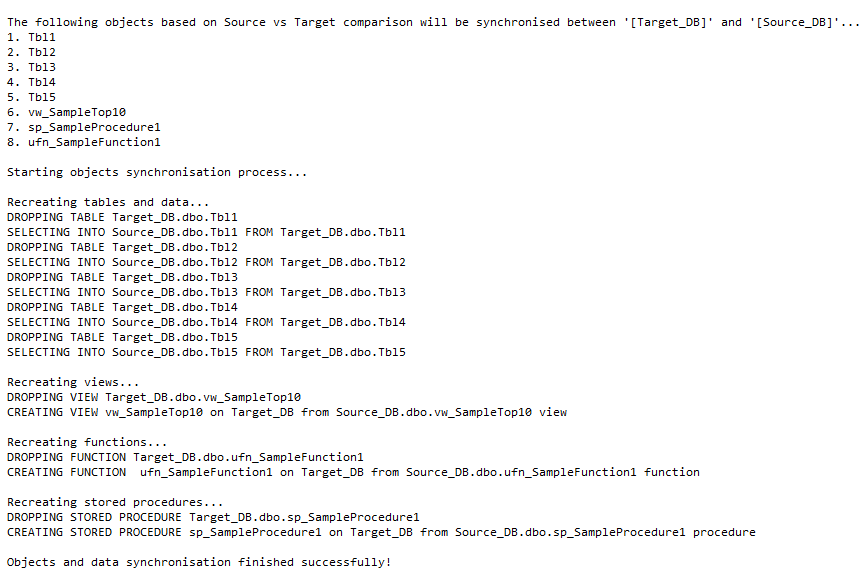
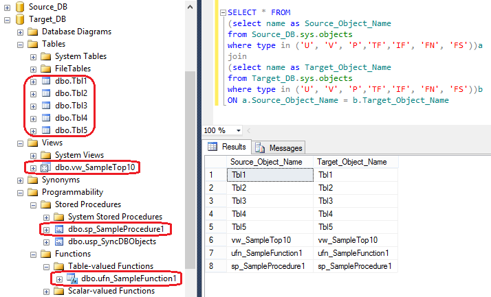
When the procedure has finished executing, both Source_DB and Target_DB should contain identical data and objects schema for tables, functions, stored procedures and tables as per execution log and each database sys.objects query image below.
 If the schema is to remain static and you only wish to synchronise data, please check out my other two posts (HERE and HERE) where I explored the dynamic functionality of cross-table data replication through on-the-fly MERGE statement creation and UPSERT execution.
Posted in: How To's, SQL
Tags: SQL, SQL Server
September 27th, 2013 / No Comments » / by admin
A few months ago I started playing around with a bunch of statistical applications and built a very simple Twitter sentiment analysis engine for feeds classification using RapidMiner – you can see the full post HERE. Since then I have been quite busy and haven’t had a chance to play with data mining applications any further but given my recent time off work and a few extra hours on my hands I was eager to replicate a proof-of-concept solution I built a long time ago for a marketing department in response to their issue with customer classification for catalogue mail-out. For that project I put together a rudimentary SSIS, SSAS and SSRS solution which, in its core functionality utilised Microsoft data mining features. In this post I will show you how to build a similar solution (highly simplified though – no reporting or complex ETL/data cleansing features) using Excel. I will also use the same dataset to compare my results to those generated by SAP Predictive Analysis – another application which I recently attended a demo of. SAP Predictive Analysis is a ‘new kid on the block’ of data mining software crated to allow analysts and business users, not quants with PhDs, to build simple models to gather insight from their data.
Excel, being the lovechild of any commercial department can be utilised as a powerful tool for many different domains of data mining, especially in conjunction with Analysis Services engine running as part of Microsoft SQL Server deployment. Yes, it is true that Excel contains many mathematical and statistical functions, however, on its own, Excel does not provide the functionality for robust data cleansing, model testing, scripting languages such as DMX, deployment options etc. which can be achieved in conjunction with SQL Server engine. Also, in order to take advantage of the highly simplified data mining techniques mostly driven by step-by-step wizard dialogs, Excel requires a connection to Analysis Services so if you’re keen to replicate this exercise in your own environment, make sure you can connect to SSAS database and have Excel data mining add-in installed.
Let’s go ahead and start with a problem definition to help us determine the possible course of action and two sample datasets – one for model training and another one which will be used for scoring.
Problem Definition
Let’s envisage that a telecom company has struck a deal with a telephone manufacturer and is about to release a new model of a highly anticipated smart phone on a competitive plan. They know that the phone is going to be a hit among its customers but given that their marketing department is very cutting-edge and would like to maximise the odds of addressing advertising campaign budget towards the right group of clients, they want to use the customer data to pinpoint those individuals who are happy not to upgrade their existing phones. Chances are that there will almost certainly be a large group of die-hard fans who are even happy to camp outside the store just to be the first ones to get their hands on the latest gadget when it eventually gets released – these individuals do not need the power of persuasion or marketing dollars spent on. It’s the ones who are on the fence, undecided or doubtful that may need just a little nudge to sway them over the line. This group will unknowingly become the focus of the campaign but in order to determine their profile, we first must determine the method we can employ to single out customers who fall into this category.
The decision tree is probably the most popular data mining technique because of fast training performance, a high degree of accuracy, and easily understandable patterns. The most common data mining task for a decision tree is classification — that is, determining whether or not a set of data belongs to a specific type, or class. For example, loan applicants can be classified as high risk or low risk, and decision trees help determine the rules to perform that classification based on historical data. The principal idea of a decision tree is to split your data recursively into subsets. Each input attribute is evaluated to determine how cleanly it divides the data across the classes (or states) of your target variable (predictable attribute). The process of evaluating all inputs is then repeated on each subset. When this recursive process is completed, a decision tree is formed. For this exercise I will use Microsoft decision trees algorithm as it fits the intended classification purpose very well. There is lots of information on the internet pertaining to decision tree algorithm applications so rather than theorising, let’s look at some concrete examples of data that will be used for this post.
Let’s assume that marketing department has provided us with a training dataset (downloadable HERE) of customers (identified with unique IDs for privacy reasons) in conjunction with a series of additional attributes such as Gender, Age, Marital Status, Contract Length, whether the customer has kids, whether he or she is married etc. Amongst all those there is also one attribute – Adopter Class – which categorises clients based on whether they are likely to adopt the new product relatively quickly after it has been released or whether they are happy to wait. This attribute has four distinctive values – Late, Very Late, Early, Very Early – which indicate customer adoption promptness. Obviously, if a customer has been tagged with Very Early in the past based on their previous behaviour patterns, he or she is highly likely to procure a new phone the moment it becomes available. On the other side of the spectrum are those customers marked as Very Late, meaning they are not as savvy to peruse the latest and greatest and are happy to wait. All those attributes in the training dataset will be used to train our model to learn about the most deterministic factors that influence clients’ behaviours.
We were also given a second dataset (downloadable HERE) which contains a different set of customers with same descriptive attributes attached to their IDs but this time without Adopter Class populated. The goal is to mine the already pre-classified customers from our first dataset and based on the findings apply the ‘knowledge’ to determine the category the new set of customers will most likely fall into.
Datasets and SQL Code
As far as the individual datasets, you can download them HERE or alternatively, you can re-create them from scratch using the SQL code I wrote to populate our training and scoring dataset files as per below. Please note that if you wish to run the code yourself, ensure that you have SampleData directory created on your C:\ drive or alternatively change the code to output the files into your nominated directory structure. Also, in relation to datasets content, note that this data was synthesised using SQL and is not a true representation of the customer data in a sense that the values are not as random or representative of a group of individuals as they would be if the data was coming from a data warehouse or CRM sources.
USE [master]
GO
IF EXISTS (SELECT name FROM sys.databases WHERE name = N'Temp_DB')
BEGIN
-- Close connections to the DW_Sample database
ALTER DATABASE [Temp_DB] SET SINGLE_USER WITH ROLLBACK IMMEDIATE
DROP DATABASE [Temp_DB]
END
GO
CREATE DATABASE [Temp_DB]
GO
USE  [Temp_DB]

DECLARE @Gender Table
(Gender char(1))
DECLARE @Age Table
(Age int)
DECLARE @Marital_Status Table
(Marital_Status varchar (20))
DECLARE @Yes_No_Flag Table
(Flag char (1))
DECLARE @Current_Plan Table
(CPlan varchar (20))
DECLARE @Payment_Method Table
(Payment_Method varchar (50))
DECLARE @Contract_Length Table
(Contract_Length varchar (30))
DECLARE @Adopter_Class Table
(Adopter_Class varchar (20))
DECLARE @Age_Range Table
(Age int)

DECLARE @Years int = 18

WHILE @Years < 65
BEGIN
	INSERT INTO @Age_Range
	SELECT @Years
	SET @Years = @Years +1
END

INSERT INTO @Gender
VALUES ('M'), ('F')
INSERT INTO @Age
SELECT * FROM @Age_Range
INSERT INTO @Marital_Status
VALUES ('Married'), ('Single')
INSERT INTO @Yes_No_Flag
VALUES('Y'), ('N')
INSERT INTO @Current_Plan
VALUES ('Low'), ('Medium'), ('Heavy'), ('PrePaid')
INSERT INTO @Payment_Method
VALUES ('Automatic'), ('Non-Automatic')
INSERT INTO @Contract_Length
VALUES ('12 Months'), ('24 months'), ('36 Months'), ('No Contract')
INSERT INTO @Adopter_Class
VALUES ('Very Early'), ('Early'), ('Very Late'), ('Late')

CREATE TABLE Temp_Results
(UserID					int				NOT NULL,
Gender					char(1)			NOT NULL,
Age						int				NOT NULL,
Marital_Status			varchar (20)	NOT NULL,
Current_Plan			varchar (20)	NOT NULL,
Payment_Method			varchar (50)	NOT NULL,
Contract_Length			varchar (30)	NOT NULL,
Has_Kids				char (1)		NOT NULL,
Other_Services_Bundled	char(1)			NOT NULL,
Adopter_Class			varchar(20)		NOT NULL)

SET NOCOUNT ON
DECLARE @Random INT;
DECLARE @Upper INT;
DECLARE @Lower INT
SET @Lower = 10000
SET @Upper = 50000
DECLARE @Records_Count int = 0
WHILE @Records_Count < 5000
BEGIN
	INSERT INTO Temp_Results
	SELECT  ROUND(((@Upper - @Lower -1) * RAND() + @Lower), 0),
	(SELECT TOP (1) Gender			FROM @Gender			ORDER BY NewID()),
	(SELECT TOP (1) Age				FROM @Age				ORDER BY NewID()),
	(SELECT TOP (1) Marital_Status	FROM @Marital_Status	ORDER BY NewID()),
	(SELECT TOP (1) CPlan			FROM @Current_Plan		ORDER BY NewID()),
	(SELECT TOP (1) Payment_Method	FROM @Payment_Method	ORDER BY NewID()),
	(SELECT TOP (1) Contract_Length FROM @Contract_Length	ORDER BY NewID()),
	(SELECT TOP (1) Flag			FROM @Yes_No_Flag		ORDER BY NewID()),
	(SELECT TOP (1) Flag			FROM @Yes_No_Flag		ORDER BY NewID()),
	(SELECT TOP (1) Adopter_Class	FROM @Adopter_Class		ORDER BY NewID())
	SET @Records_Count = @Records_Count + 1
END

UPDATE Temp_Results
SET Payment_Method	=	CASE	WHEN Current_Plan = 'PrePaid'	THEN 'Non-Automatic' ELSE Payment_Method END
UPDATE Temp_Results
SET Contract_Length =	CASE	WHEN Current_Plan = 'PrePaid'	THEN 'No Contract' ELSE Contract_Length END
UPDATE Temp_Results
SET Adopter_Class	=	CASE	WHEN	Age BETWEEN 18 and 35 AND
										Other_Services_Bundled = 'Y' AND
										Current_Plan IN ('Medium', 'Heavy', 'Low') AND
										Contract_Length IN ('12 Months', '24 Months')
										THEN 'Very Early'
								WHEN	Age BETWEEN 36 and 45 AND
										Other_Services_Bundled = 'Y' AND
										Current_Plan IN ('Medium', 'Heavy', 'Low') AND
										Contract_Length IN ('12 Months', '24 Months', '36 Months')
										THEN 'Early'
								WHEN	Age BETWEEN 46 and 55 AND
										Other_Services_Bundled = 'N' AND
										Current_Plan IN ('Medium','Low') AND
										Contract_Length IN ('12 Months', '24 Months', '36 Months')
										THEN 'Late'
								WHEN	Age > 55 AND
										Other_Services_Bundled ='N' AND
										Current_PLan IN ('PrePaid', 'Low') AND
										Contract_Length IN ('No Contract', '36 Months', '24 Months')
										THEN 'Very Late' ELSE Adopter_Class END

DECLARE @ID varchar (200)
DECLARE @COUNT int
DECLARE CUR_DELETE CURSOR FOR
	SELECT UserID,COUNT([UserID]) FROM [Temp_Results]
	GROUP BY [UserID] HAVING COUNT([UserID]) > 1
	OPEN CUR_DELETE
		FETCH NEXT FROM CUR_DELETE INTO @ID, @COUNT
		WHILE @@FETCH_STATUS = 0
		BEGIN
		DELETE TOP(@COUNT -1) FROM [Temp_Results] WHERE [UserID] = @ID
		FETCH NEXT FROM CUR_DELETE INTO @ID, @COUNT
	END
CLOSE CUR_DELETE
DEALLOCATE CUR_DELETE

DECLARE
@saveloc		VARCHAR(2048),
@query			VARCHAR(2048),
@bcpquery		VARCHAR(2048),
@bcpconn		VARCHAR(64),
@bcpdelim		VARCHAR(2)

/*
To enable CMD_SHELL IF DISABLED
EXEC sp_configure 'show advanced options', 1
GO
RECONFIGURE
GO
EXEC sp_configure 'xp_cmdshell', 1
GO
RECONFIGURE
GO
*/

SET @query =	'USE Temp_DB
				SELECT
				''UserID''					as H1,
				''Gender''					as H2,
				''Age''						as H3,
				''Marital_Status''			as H4,
				''Current_Plan''			as H5,
				''Payment_Method''			as H6,
				''Contract_Length''			as H7,
				''Has_Kids''				as H8,
				''Other_Services_Bundled''	as H9,
				''Adopter_Class''			as H10
				UNION ALL
				SELECT
				CAST(UserID as Varchar(10)),
				Gender,
				CAST(Age as Varchar (10)),
				Marital_Status,
				Current_Plan,
				Payment_Method,
				Contract_Length,
				Has_Kids,
				Other_Services_Bundled,
				Adopter_Class
				FROM Temp_Results'
SET @saveloc = 'c:\SampleData\Training_DataSet.csv'
SET @bcpdelim   = ','
SET @bcpconn    = '-T' -- Trusted
--SET @bcpconn    = '-U <username> -P <password>' -- SQL authentication
SET @bcpquery = 'bcp "' + replace(@query, char(10), '') + '" QUERYOUT "' + @saveloc + '" -c -t^' + @bcpdelim + ' ' + @bcpconn + ' -S ' + @@servername
EXEC master..xp_cmdshell @bcpquery

TRUNCATE TABLE Temp_Results

ALTER TABLE Temp_Results
DROP COLUMN Adopter_Class

SET @Lower = 50001
SET @Upper = 99999
SET @Records_Count = 0
WHILE @Records_Count < 5000
BEGIN
	INSERT INTO Temp_Results
	SELECT  ROUND(((@Upper - @Lower -1) * RAND() + @Lower), 0),
	(SELECT TOP (1) Gender			FROM @Gender			ORDER BY NewID()),
	(SELECT TOP (1) Age				FROM @Age				ORDER BY NewID()),
	(SELECT TOP (1) Marital_Status	FROM @Marital_Status	ORDER BY NewID()),
	(SELECT TOP (1) CPlan			FROM @Current_Plan		ORDER BY NewID()),
	(SELECT TOP (1) Payment_Method	FROM @Payment_Method	ORDER BY NewID()),
	(SELECT TOP (1) Contract_Length FROM @Contract_Length	ORDER BY NewID()),
	(SELECT TOP (1) Flag			FROM @Yes_No_Flag		ORDER BY NewID()),
	(SELECT TOP (1) Flag			FROM @Yes_No_Flag		ORDER BY NewID())
	SET @Records_Count = @Records_Count + 1
END

SET @ID =''
SET @COUNT = 0
DECLARE CUR_DELETE CURSOR FOR
	SELECT UserID,COUNT([UserID]) FROM [Temp_Results]
	GROUP BY [UserID] HAVING COUNT([UserID]) > 1
	OPEN CUR_DELETE
		FETCH NEXT FROM CUR_DELETE INTO @ID, @COUNT
		WHILE @@FETCH_STATUS = 0
		BEGIN
		DELETE TOP(@COUNT -1) FROM [Temp_Results] WHERE [UserID] = @ID
		FETCH NEXT FROM CUR_DELETE INTO @ID, @COUNT
	END
CLOSE CUR_DELETE
DEALLOCATE CUR_DELETE

SET @query =	'USE Temp_DB
				SELECT
				''UserID''					as H1,
				''Gender''					as H2,
				''Age''						as H3,
				''Marital_Status''			as H4,
				''Current_Plan''			as H5,
				''Payment_Method''			as H6,
				''Contract_Length''			as H7,
				''Has_Kids''				as H8,
				''Other_Services_Bundled''	as H9
				UNION ALL
				SELECT
				CAST(UserID as Varchar(10)),
				Gender,
				CAST(Age as Varchar (10)),
				Marital_Status,
				Current_Plan,
				Payment_Method,
				Contract_Length,
				Has_Kids,
				Other_Services_Bundled
				FROM Temp_Results'
SET @saveloc = 'c:\SampleData\Scoring_DataSet.csv'
SET @bcpdelim   = ','
SET @bcpconn    = '-T' -- Trusted
--SET @bcpconn    = '-U <username> -P <password>' -- SQL authentication
SET @bcpquery = 'bcp "' + replace(@query, char(10), '') + '" QUERYOUT "' + @saveloc + '" -c -t^' + @bcpdelim + ' ' + @bcpconn + ' -S ' + @@servername
EXEC master..xp_cmdshell @bcpquery

DROP TABLE Temp_Results
Decision Trees Model Deployment and Application
Once the two files have been created (or saved if you opted out of running the script and just downloaded them), we can open the one prefixed with ‘training’ and highlight all records. Having data mining plug-in installed, Classify button should be one of the options available form Data Mining tab on Excel’s ribbon. Clicking it should start the wizard which will take us through the steps where we will adjust model’s properties and variables before deployment.
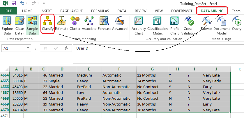
Step one provides a brief description of its features and functionality, let’s click Next and to proceed to data range selection dialog. As per image above you will notice that I have selected over 4600 records generated by the SQL query. Alternatively, you can also select external data source. Let’s click Next to advance to Classification window where we have an option to choose the columns participating in the model creation as well as the column to analyse. I have intentionally removed the UserID column which has no relevance or dependencies on other columns and selected Adopter_Class column as an analysis target. Adopter_Class column contains the data which is the focus of this exercise and marketing wants to know how this attribute gets affected by other columns’ data.
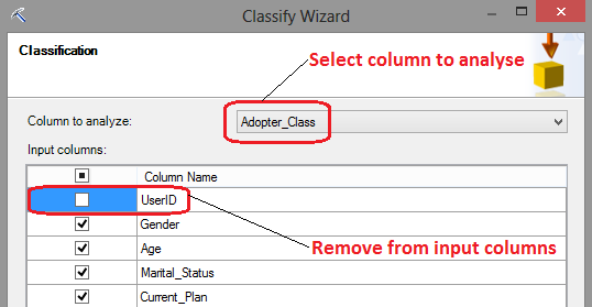
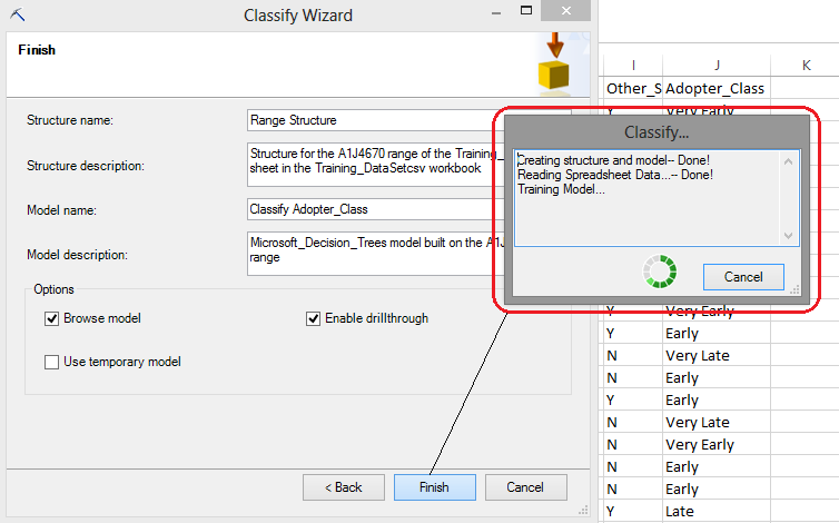
Clicking Next we will advance to Split Data Into Training And Testing step where we can specify the percentage of our dataset to get allocated to training and testing the model. We will leave this value at default and advance to the last step where we have an option to change some of the final properties such as Model Name or Model Description. Again, we will leave everything at default and finish the wizard deploying the model as per image below.
After data reading and training has completed and our decision trees model has been deployed we can see the breakdown of individual attributes participating in how their values and affinities or dependencies relate to Adopter Class values. In the below image, the Background property has been set to Very Late, which is the group marketing campaign wants to potentially address when devising their next campaign. These people are the most resistant to adopting new technology and with the release of the new smart phone, marketing is hoping to gather insight into their profile. Rectangles shaded in darkest blue are representative of the target group i.e. very late adopters (click on image to enlarge).
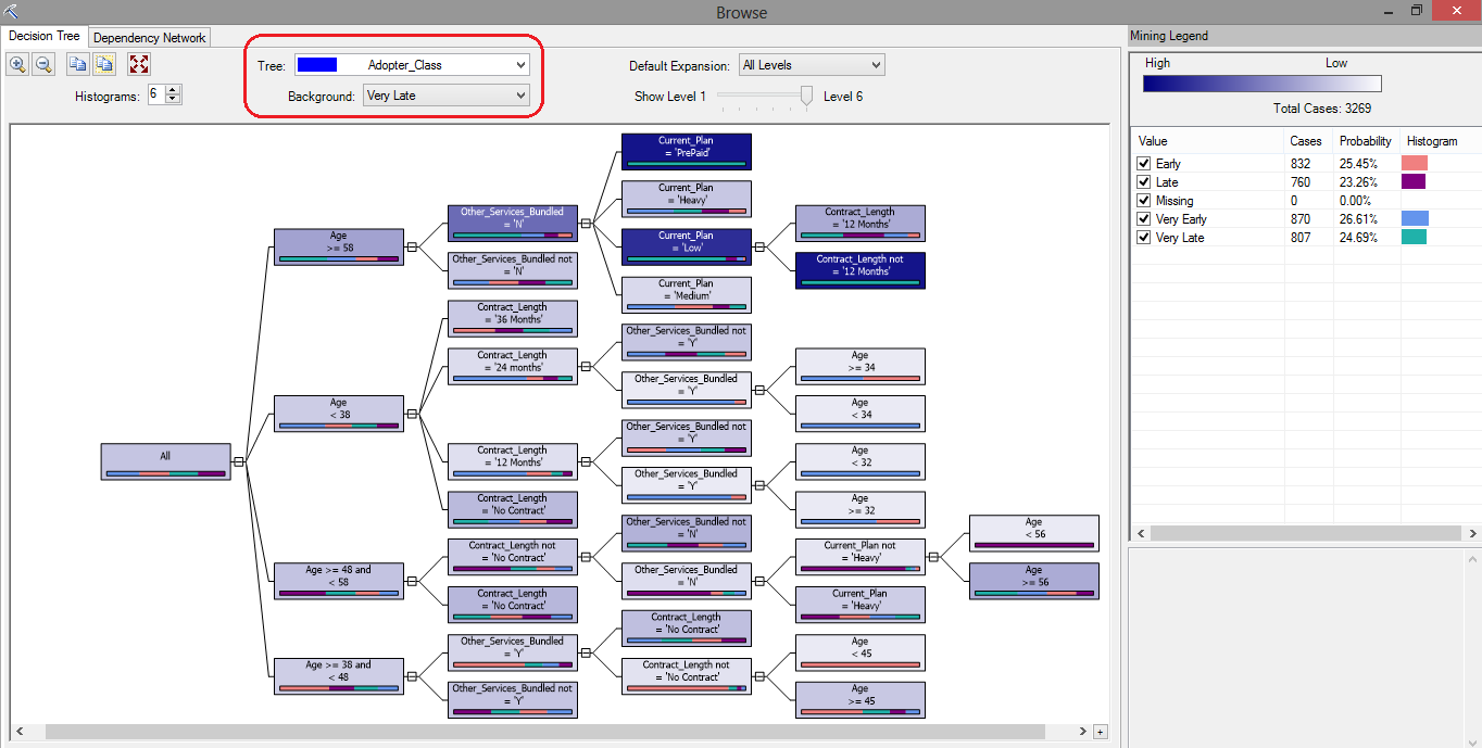
Following this tree from left to right, we can deduce the following.
- Individuals who are 58 or older, with no other services bundled, on a Pre-paid plan fall into Vary Late adopters category.
- Individuals who are 58 or older, with no other services bundled, on a Low plan and not on a 12 months contract fall into Very Late adopters category.
If we were to review the profile of customers opposite to very late adopters i.e. individuals how are keen to update sooner and more frequently, the model would look as per below (click on image to enlarge).
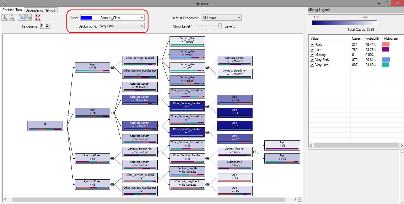
This tree diagram indicates that it’s the customers who are likely to be less than 38 years old, with other services bundled and on either 24 or 12 months contracts who are the most likely ones to crave new technology.
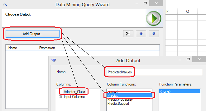
That is all well and god but how can apply this knowledge to our other customers? As you remember, our second dataset contains another group of individuals who have not been classified as yet. The ultimate purpose of this type of exercise is to apply such model to another group of clients and predict with a certain level of confidence what category they may fall into, based on their attributes’ values and what our model has ‘learnt’. Let’s apply this knowledge to our scoring dataset and open up the second file the script has generated – Scoring_DataSet.csv file. After highlighting all records and columns let’s execute the data mining DMX query clicking on the Query button which starts another wizard. In step number 2 of the wizard (first one is just a process description) we can select the model we have just deployed and proceeding through steps 3 and 4 we have an option to select the data source and specify columns relationships. Let’s leave those with default options selected i.e. data source will be the data range selected previously and columns relationships will be mapped out automatically for us and advance to adding an output column step. Here, we will proceed as per the image below.
When completed, click OK and Next to advance to the next step where we have an option to choose a destination for the query result. Let’s go ahead and select Append To The Input Data from the options provided and click Finish to let Excel and DMX query which has built in the background run our scoring data through the model to determine the Adopter Class output for each observation. When finished, we should be presented with an additional column added to our workbook which indicates which category decision tree model we applied to this dataset ‘thinks’ the customer should belong to.
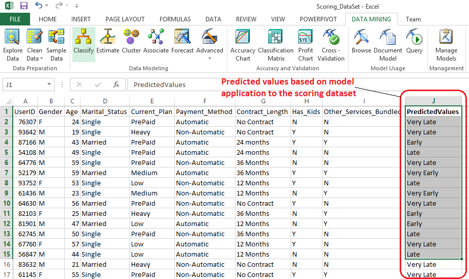
If we filter this dataset on the records with adopter class equal to Very Late, we would effectively shrink our data to a quarter of the original size allowing the business to make conscious and data-backed decision on who to direct the marketing campaign to. Not only does this approach prevent a ‘stab-in –the-dark’ approach but it can also allow the business to save a lot of money e.g. if campaign was relying on printing special offers catalogues etc. Based on this final list marketing can correlate customer ids with other customer descriptive attributes such as addresses, names, email address or location coordinates to drive the campaign dollars further.
Just as a reference, I also compared the output from the model with another application capable of classifying based on decision tree algorithm – SAP Predictive Analysis. After installing R to integrate R_CNR Tree algorithm I re-created the model and this is what it appeared as (click on image to enlarge).
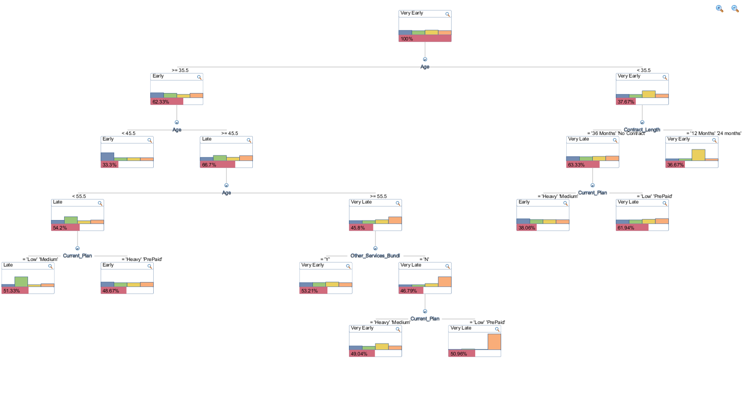
Arguably, I think that Excel output is much easier to read, analyse and interpret, especially that it provides a filtering option to highlight the groups of interests rather simply relying on color-coding. Also, as a secondary exercise I run the scoring dataset through the newly created model in SAP Predictive Analytics, outputting the newly tagged data into a separate file for the purpose of comparison (you can download all the files from HERE).

Quick, analysis revealed that out of close to 5000 records, overlapping results constituted around 55 percent or nearly 2600 observations. That means that for nearly half of all the records analysed the results varied depending on which application was used i.e. Excel with SSAS or SAP’s Predictive Analysis. Also, for comparison, I run the predicted values through Classification Matrix and Accuracy Chart tools to evaluate the models performance for false positive, true positive, false negative, and true negative. Given that I only run it in Excel, predicted data produced by Excel was 100 percent spot on whereas SAP’s Predictive Analysis output was a complete hit and miss (you can look at the results in the ‘Quick Analysis SAP vs Excel’ spreadsheet HERE). These are pretty dramatic variances and without further investigation I would be hesitant to provide a definite answer as to why these discrepancies are so large but chances are these tools and their corresponding algorithms differ in how they handle the data even though they both bear the same name – Decision Trees. This only reinforces the premise that data mining tools and the results they produce, as easy and fool-proof as they may seem on the face value, need to be treated with caution and consideration. Sometimes, depending on variables such as the data we use, applied algorithm and associated parameters, mining application etc. the results can vary significantly hence requiring more extensive analysis and interpretation.
Posted in: Data Mining, Excel, How To's
Tags: Data Mining, Excel, SAP, SSAS
 If the schema is to remain static and you only wish to synchronise data, please check out my other two posts (HERE and HERE) where I explored the dynamic functionality of cross-table data replication through on-the-fly MERGE statement creation and UPSERT execution.


Never thought Polybase could be used in this capacity and don't think Microsoft advertised this feature (off-loading DB data as…