Kicking the tires on BigQuery – Google’s Serverless Enterprise Data Warehouse (Part 2)
Note: Part 1 can be found HERE.
TPC-DS Benchmark Continued…
In the previous post I outlined some basic principles around Google’s BigQuery architecture as well as a programmatic way to interact with TPC-DS benchmark data set (files prep, staging data on Google cloud storage bucket, creating datasets and tables schema, data loading etc). In this post I will go through a few analytical queries defined as part of the comprehensive, 99-queries-based TPC-DS standard and their execution patterns (similar to the blog post I wrote on spinning up a small Vertica cluster HERE) and look at how BigQuery integrates with the likes of Tableau and PowerBI, most likely the top two applications used nowadays for rapid data analysis.
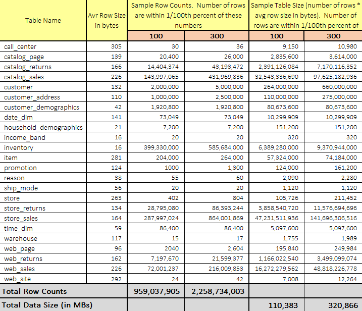
Firstly, let’s see how BigQuery handles some of the TPC-DS queries running across 100GB and 300GB dataset comprised of 24 tables and over 2 billion rows collectively (300GB dataset). As with the previous blog posts depicting TPC-DS queries execution on a Vertica platform HERE, the following image depicts row numbers and data size distribution for this exercise.
For this exercise, I run a small Python script executing the following queries from the standard TPC-DS benchmark suite: 5, 10, 15, 19, 24, 27, 33, 36, 42, 45, 48, 54, 58, 60, 65, 68, 73, 78, 83, 85, 88, 93, 96, 99. The script sequentially executes TPC-DS SQL commands stored in an external file reporting execution times each time a query is run. All scripts used for this project can be found in my OneDrive folder HERE.
#!/usr/bin/python
import configparser
import sys
from os import path, remove
from time import time
from google.cloud import bigquery

config = configparser.ConfigParser()
config.read("params.cfg")

bq_tpc_ds_sql_statements_file_path = config.get(
    "Files_Path", path.normpath("bq_tpc_ds_sql_statements_file_path"))
bq_client = config.get("Big_Query", path.normpath("bq_client"))
bq_client = bigquery.Client.from_service_account_json(bq_client)


def get_sql(bq_tpc_ds_sql_statements_file_path):
    """
    Source operation types from the tpc_ds_sql_queries.sql SQL file.
    Each operation is denoted by the use of four dash characters
    and a corresponding query number and store them in a dictionary
    (referenced in the main() function).
    """
    query_number = []
    query_sql = []

    with open(bq_tpc_ds_sql_statements_file_path, "r") as f:
        for i in f:
            if i.startswith("----"):
                i = i.replace("----", "")
                query_number.append(i.rstrip("\n"))

    temp_query_sql = []
    with open(bq_tpc_ds_sql_statements_file_path, "r") as f:
        for i in f:
            temp_query_sql.append(i)
        l = [i for i, s in enumerate(temp_query_sql) if "----" in s]
        l.append((len(temp_query_sql)))
        for first, second in zip(l, l[1:]):
            query_sql.append("".join(temp_query_sql[first:second]))
    sql = dict(zip(query_number, query_sql))
    return sql


def run_sql(query_sql, query_number):
    """
    Execute SQL query as per the SQL text stored in the tpc_ds_sql_queries.sql
    file by it's number e.g. 10, 24 etc. and report returned row number and
    query processing time
    """
    query_start_time = time()
    job_config = bigquery.QueryJobConfig()
    job_config.use_query_cache = False
    query_job = bq_client.query(query_sql, job_config=job_config)
    rows = query_job.result()
    rows_count = sum(1 for row in rows)
    query_end_time = time()
    query_duration = query_end_time - query_start_time
    print("Query {q_number} executed in {time} seconds...{ct} rows returned.".format(
        q_number=query_number, time=format(query_duration, '.2f'), ct=rows_count))


def main(param, sql):
    """
    Depending on the argv value i.e. query number or 'all' value, execute
    sql queries by calling run_sql() function
    """
    if param == "all":
        for key, val in sql.items():
            query_sql = val
            query_number = key.replace("Query", "")
            run_sql(query_sql, query_number)
    else:
        query_sql = sql.get("Query"+str(param))
        query_number = param
        run_sql(query_sql, query_number)


if __name__ == "__main__":
    if len(sys.argv[1:]) == 1:
        sql = get_sql(bq_tpc_ds_sql_statements_file_path)
        param = sys.argv[1]
        query_numbers = [q.replace("Query", "") for q in sql]
        query_numbers.append("all")
        if param not in query_numbers:
            raise ValueError("Incorrect argument given. Looking for <all> or <query number>. Specify <all> argument or choose from the following numbers:\n {q}".format(
                q=', '.join(query_numbers[:-1])))
        else:
            param = sys.argv[1]
            main(param, sql)
    else:
        raise ValueError(
            "Too many arguments given. Looking for 'all' or <query number>.")
The following charts depicts queries performance based on 100GB and 300GB datasets with BigQuery cache engaged and disengaged. As BigQuery, in most cases, writes all query results (including both interactive and batch queries) to a table for 24 hours, it is possible for BigQuery to retrieve the previously computed results from cache thus speeding up the overall execution time.
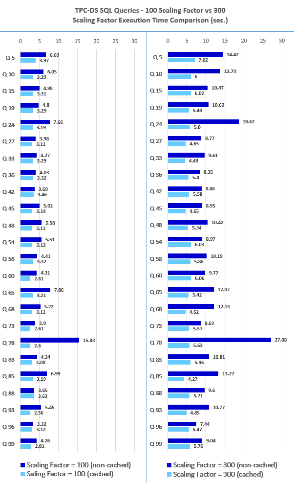
While these results and test cases are probably not truly representative of the ‘big data’ workloads, they provide a quick snapshot of how traditional analytical workloads would perform on the BigQuery platform. Scanning large tables with hundreds of millions of rows seemed to perform quite well (especially cached version) and performance differences between 100GB and 300GB datasets were consistent with the increase in data volumes. As BigQuery does not provide many ‘knobs and switches’ to tune queries based on their execution pattern (part of its no-ops appeal), there is very little room for improving its performance beyond avoiding certain anti-patterns. The ‘execution details’ pane provides some diagnostic insight into the query plan and timing information however, many optimizations happen automatically, which may differ from other environments where tuning, provisioning, and monitoring may require dedicated, knowledgeable staff. I believe that for similar data volumes, much faster runtimes are possible if run on a different OLAP database from a different vendor (for carefully tuned and optimised queries), however, this will imply substantial investment in the upfront infrastructure setup and specialised resources, which for a lot of companies will negate the added benefits and possibly impair time-to-market competitive advantage.
Looking at some ad hoc queries execution through Tableau, the first thing I needed to do was to create a custom SQL to slice and dice TPC-DS data as Tableau ‘conveniently’ hides attributes with NUMERIC data type (unsupported at this time in Tableau). Casting those to FLOAT64 data type fixed the issue and I was able to proceed with building a sample dashboard using the following query.
SELECT CAST(store_sales.ss_sales_price AS FLOAT64) AS ss_sales_price,
       CAST(store_sales.ss_net_paid AS FLOAT64)    AS ss_net_paid,
       store_sales.ss_quantity,
       date_dim.d_fy_quarter_seq,
       date_dim.d_holiday,
       item.i_color,
       store.s_city,
       customer_address.ca_state
FROM tpc_ds_test_data.store_sales
         JOIN tpc_ds_test_data.customer_address ON
    store_sales.ss_addr_sk = customer_address.ca_address_sk
         JOIN tpc_ds_test_data.date_dim ON
    store_sales.ss_sold_date_sk = date_dim.d_date_sk
         JOIN tpc_ds_test_data.item ON
    store_sales.ss_item_sk = item.i_item_sk
         JOIN tpc_ds_test_data.store ON
    store_sales.ss_store_sk = store.s_store_sk
Running a few analytical queries across the 300GB TPC-DS dataset with all measures derived from its largest fact table (store_sales) BigQuery performed quite well, with majority of the queries taking less than 5 seconds to complete. As all queries executed multiple times are cached, I found BigQuery response even faster (sub-second level response) when used with the same measures, dimensions and calculations repetitively. However, using this engine for an ad-hoc exploratory analysis in a live/direct access mode can become very expensive, very quickly. The few queries run (73 to be exact) as part of this demo (see footage below) cost me over 30 Australia dollars on this 300GB dataset. I can only imagine how much it would cost to analyse much bigger dataset in this manner, so unless analysis like this can be performed on an extracted dataset, I find it hard to recommend as a rapid-fire, exploratory database engine for an impromptu data analysis.
BigQuery Machine Leaning (BQML)
As more and more data warehousing vendors jump on the bandwagon of bringing data science capability closer to the data, Google is also trying to cater for analysts who predominantly operate in the world of SQL by providing a simplified interface for a machine learning models creation. This democratizes the use of ML by empowering data analysts, the primary data warehouse users, to build and run models using existing business intelligence tools and spreadsheets. It also increases the speed of model development and innovation by removing the need to export data from the data warehouse.
BigQuery ML is a series of SQL extensions that allow data scientists to build and deploy machine learning models that use data stored in the BigQuery platform, obfuscating many of the painful and highly mathematical aspects of machine learning methods into simple SQL statements. BigQuery ML is a part of a much larger ecosystem of Machine Learning tools available on Google Cloud.
The current release (as of Dec. 2018) only supports two types of machine learning models.
- Linear regression – these models can be used for predicting a numerical value representing a relation variables e.g. between customer waiting (queue) time and customer satisfaction.
- Binary logistic regression – these models can be used for predicting one of two classes (such as identifying whether an email is spam).
Developers can create a model by using the CREATE or CREATE OR REPLACE MODEL or CREATE MODEL IF NOT EXISTS syntax (presently, the size of the model cannot exceed 90 MB). A number of parameters can be passed (some optional), dictating model type, name of label column, regularization technique etc.
Looking at a concrete example, I downloaded the venerable and widely used by many aspiring data scientists Titanic Kaggle dataset. It contains training data for 891 passengers and provides information on the fate of passengers on the Titanic, summarized according to economic status (class), sex, age etc. and is the go-to dataset for predicting passenger survivability based on those features. Once the data is loaded into two separate tables – test_data and train_data – creating a simple model is as easy as creating a database view. We can perform binary classification and create a sample logistic regression model with the following syntax.
CREATE MODEL
  `bq_ml.test_model`
OPTIONS
  (model_type = 'logistic_reg',
  input_label_cols = ['Survived'],
  max_iterations=10) AS
SELECT
  *
FROM
  bq_ml.train_data
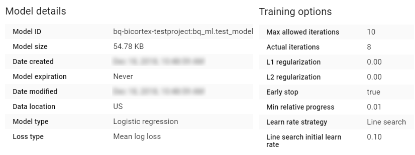
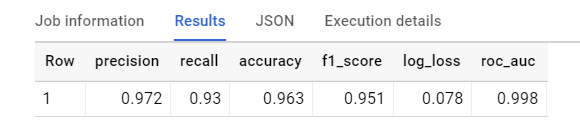
Once the model has been created we can view its details and training options in BigQuery as per the image below.
Now that we have a classifier model created on our data we can evaluate it using ML.EVALUATE function.
SELECT
  *
FROM
  ML.EVALUATE (MODEL `bq_ml.test_model`,
    (
  SELECT
    *
  FROM
    `bq_ml.train_data`),
    STRUCT (0.55 AS threshold))
This produces a single row of evaluation parameters e.g. accuracy, recall, precision etc. which allow us to determine model performance.
We can also use the ML.ROC_CURVE function to evaluate logistic regression models, but ML.ROC_CURVE is not supported for multiclass models. Also, notice the optional threshold parameter which is a custom threshold for this logistic regression model to be used for evaluation. The default value is 0.5. The threshold value that is supplied must be of type STRUCT. A zero value for precision or recall means that the selected threshold produced no true positive labels. A NaN value for precision means that the selected threshold produced no positive labels, neither true positives nor false positives. If both table_name and query_statement are unspecified, you cannot use a threshold. Also, threshold cannot be used with multiclass logistic regression models.
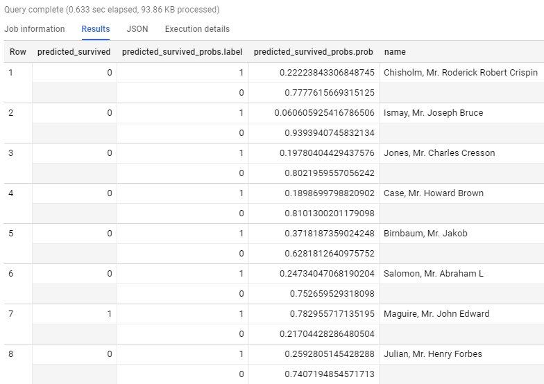
Finally, we can use our model to predict who survived the Titanic disaster by applying our trained model to the test data. The output of the ML.PREDICT function has as many rows as the input table, and it includes all columns from the input table and all output columns from the model. The output column names for the model are predicted_ and (for logistic regression models) predicted__probs. In both columns, label_column_name is the name of the input label column used during training. The following query generates the prediction – 1 for ‘survived’ and 0 for ‘did not survive’, the probability and the name of the passengers on the ship.
SELECT
  predicted_survived,
  predicted_survived_probs,
  name
FROM
  ML.PREDICT (MODEL `bq_ml.test_model`,
    (
  SELECT
    *
  FROM
    `bq_ml.test_data`))
When executed, we can clearly see the prediction for each individual passenger name.
Conclusion
Why Use the Google Cloud Platform? The initial investment required to import data into the cloud is offset by some of the advantages offered by BigQuery. For example, as a fully-managed service, BigQuery requires no capacity planning, provisioning, 24×7 monitoring or operations, nor does it require manual security patch updates. You simply upload datasets to Google Cloud Storage of your account, import them into BigQuery, and let Google’s experts manage the rest. This significantly reduces your total cost of ownership (TCO) for a data handling solution. Growing datasets have become a major burden for many IT department using data warehouse and BI tools. Engineers have to worry about so many issues beyond data analysis and problem-solving. By using BigQuery, IT teams can get back to focusing on essential activities such as building queries to analyse business-critical customer and performance data. Also, BigQuery’s REST API enables you to easily build App Engine-based dashboards and mobile front-ends.
On the other hand, BigQuery is no panacea for all your BI issues. For starters, its ecosystem of tools and supporting platforms it can integrate with is substandard to that of other cloud data warehouse providers e.g. Amazon’s Redshift. To execute the queries from a sample IDE (DataGrip), it took me a few hours to configure a 3rd party ODBC driver (Google leaves you in the cold here) as BigQuery currently does not offer robust integration with any enterprise tool for data wrangling. Whilst Google has continually tried to reduce number of limitations and improve BigQuery features, the product has a number of teething warts which can be a deal breaker for some e.g. developers can’t rename, remove or change the type of a column (without re-writing the whole table), there is no option to create table as SELECT, there are two different SQL dialects etc. These omissions are small and insignificant in the grand scheme of things, however, touting itself as an enterprise product with those simple limitations in place is still a bit of a misnomer. Finally, BigQuery’s on-demand usage-based pricing model can be difficult to work with from procurement point of view (and therefore approved by the executives). Because there is no notion of instance type, you are charged by storage, streaming inserts and queries, which is unpredictable and may put some teams off (Google recently added Cost Control feature to partially combat this issue). Finally, Google’s nebulous road-map for the service improvements and features implementation, coupled with its sketchy track record for sun-setting its products if they do not they generate enough revenue (most big enterprises want stability and long-term support guarantee) do not inspire confidence.
All in all, as it is the case with the majority of big data vendors, any enterprise considering its adoption will have to weight up all the pros and cons the service comes with and decide whether they can live with BigQuery’s shortcomings. No tool or service is perfect but for those which have limiting dev-ops capability and want true, serverless platform capable of processing huge volumes of data very fast, BigQuery presents an interesting alternative to the current incumbents.
http://scuttle.org/bookmarks.php/pass?action=addThis entry was posted on Friday, March 1st, 2019 at 9:23 am and is filed under Cloud Computing, Programming. You can follow any responses to this entry through the RSS 2.0 feed. You can leave a response, or trackback from your own site.


admin January 27th, 2020 at 9:03 pm
Thanks mate
Martin