Vertica MPP Database Overview and TPC-DS Benchmark Performance Analysis (Part 1)
Note: Post 2 can be found HERE, Post 3 HERE and Post 4 HERE
Introduction
I have previously covered Massively Parallel Processing (MPP) databases and their preliminary benchmark numbers before e.g. AWS Redshift HERE and Azure SQL DW HERE. Both of those cloud juggernauts are touting their platforms as the logical next step in big data computation and storage evolution, leaving old-guard, legacy vendors such as Teradata and Netezza with a hard choice: shift into cloud or cloud-first operating model or be remembered in the database hall of fame of now defunct and obsolete technologies.
With this hard ultimatum, many vendors are desperately trying to pivot or at least re-align their offering with the even more demanding business expectations and provide a point of differentiation in this competitive market. For example, one of the most prominent MPP vendor, Pivotal, decided to open source its Greenplum platform under the Apache Software 2.0 license. Vertica, another large MPP market player, although still very much a proprietary platform, allows freedom of environment (no cloud lock-in) with an option of running on commodity hardware (just like Greenplum) as well as comprehensive in-database Machine Learning capabilities. Vertica also offers free usage with up to three nodes and 1TB of data and very sophisticated database engine with plenty of bells, knobs and whistles for tuning and control. Doing some digging around what experience others have had with this technology, Vertica’s database engine seems to easily match, if not surpass that of many other providers in MPP market in terms of number of features and the breadth of flexibility it provides. It is said to scale well in terms of number of concurrent users and offers a competitive TCO and cost per query (pricing license cost, storage, compute resources on a VCP e.g. AWS or Azure etc.). As someone on Quora eloquently put it when contrasting it with its biggest competitor, AWS Redshift, ‘Vertica is a magical sword. Redshift is a giant club. It doesn’t take a lot of skill to use that giant club and it can do massive crunching. But I’d rather be the wizard-ninja’ Vertica’s pedigree only seems to be amplified by the fact it was founded by Michael Stonebraker, perhaps the most prominent database pioneer and the recipient of Turing Award aka ‘Nobel prize in computing’, who also founded other database software e.g. Ingres, VoltDB or the ubiquitous PostgreSQL.
Vertica RDBMS is still very much a niche player in terms of the market share, however, given that the likes of Facebook, Etsy, Guess or Uber have entrusted their data in Vertica’s ability to deliver on enterprise analytics, it certainly deserves more attention. With that in mind I would like to outline some of Vertica’s core architectural components and conduct a small performance comparison on the dataset used for TPC-DS benchmarking across one and three nodes. This post will introduce Vertica’s key architectural and design components, with Post 2 focusing on Vertica’s installation and configuration process on a number of commodity machines. Finally, in Post 3 and Post 4 I will run some TPC-DS benchmark queries to test its performance across the maximum number of nodes allowed for the Community Edition. If you’re only interested in the benchmark outcomes you can jump into Post 3 right away.
Vertica Key Architecture Components Primer
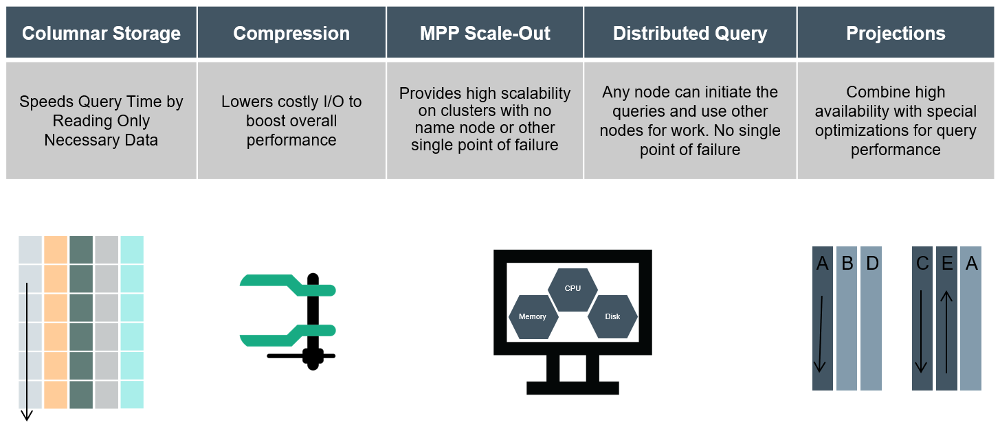
Vertica’s appeal, outside features such as ACID transactions, being ANSI-SQL compliant, high availability etc. is manly driven by its database engine optimisation for executing complex analytical queries fast. Analytic workloads are characterised by large data sets and small transaction volumes (10s-100s per second), but high number of rows per operation. This is very different to typical transactional workloads associated with the majority of legacy RDBMS applications, which can be characterised by a large number of transitions per second, where each transaction involves a handful of tuples. This performance is primarily based off of a number of technologies and design goals which facilitate this capability, most important being columnar storage, compression and MPP scale-out architecture.
Touching on some of those key points above, the following provides a quick overview of these technologies which form an integral part of its architecture.
Columnar Data Storage
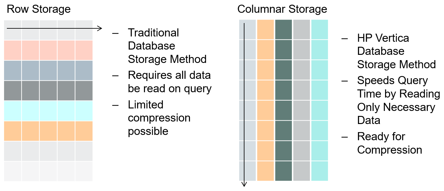
MPP databases differ from traditional transactional, row-oriented databases e.g. PostgreSQL or MySQL where data is stored and manipulated in rows. Row-based operations work really well in an application context, where the database load consists of relatively large numbers of CRUD-operations (create, read, update, delete). In analytical contexts, where the workload consists of a relatively small number of queries over a small number of columns but large numbers of records, the row based approach is not ideal. Columnar databases have been developed to work around the limitations of row-based databases for analytical purposes. They store data compressed and per column, much like an index in a row-based database reducing disk I/O as only the columns required to answer the query are read.
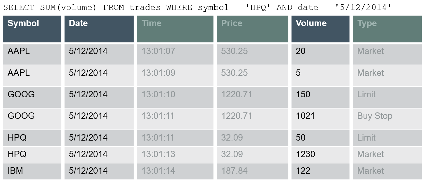
The following example depicts how a simple query can take advantage of columnar storage. In a typical, row-based RDBMS all rows, in all tables included in the query would need to be read in order to retrieve its results, regardless how wide the rows are or how many columns are required to satisfy the results output. In contrast, Vertica utilises a concept of projections – a columns based structure. Given that we only reference three columns – symbol, date and volume – only these columns need to be read from disk.
Given that majority of legacy RDBMS systems were built for data collection, not data retrieval, the columnar data storage facilitates analytical queries execution speed by avoiding scanning the data not referenced in the query itself.
Vertica also sorts data prior to storage. Queries make use of the sortedness of the data by skipping rows which would be filtered out by predicates (in a manner similar to clustered B-Tree indexes). Sorting can also be used to optimise join and aggregation algorithms.
Data Encoding And Compression
Vertica uses sophisticated encoding and compression technologies to optimize query performance and reducing storage footprint. Encoding converts data into a standard format to decrease disk I/O during query execution and reducing storage requirements. Vertica uses a number of different encoding strategies, depending on column data type, table cardinality, and sort order. Different columns in the projection may have different encodings and the same column may have a different encoding in each projection in which it appears. Vertica employs the following encoding types:
- AUTO – this encoding is ideal for sorted, many-valued columns such as primary keys. It is also suitable for general purpose applications for which no other encoding or compression scheme is applicable. Therefore, it serves as the default if no encoding/compression is specified.
- BLOCK_DICT – each block of storage, Vertica compiles distinct column values into a dictionary and then stores the dictionary and a list of indexes to represent the data block.BLOCK_DICT is ideal for few-valued, unsorted columns where saving space is more important than encoding speed. Certain kinds of data, such as stock prices, are typically few-valued within a localized area after the data is sorted, such as by stock symbol and timestamp, and are good candidates for BLOCK_DICT. By contrast, long CHAR/VARCHAR columns are not good candidates for BLOCK_DICT encoding. BLOCK_DICT encoding requires significantly higher CPU usage than default encoding schemes. The maximum data expansion is eight percent (8%).
- BLOCKDICT_COMP – this encoding type is similar to BLOCK_DICT except dictionary indexes are entropy coded. This encoding type requires significantly more CPU time to encode and decode and has a poorer worst-case performance. However, if the distribution of values is extremely skewed, using BLOCK_DICT_COMP encoding can lead to space savings.
- BZIP_COMP – BZIP_COMP encoding uses the bzip2 compression algorithm on the block contents. This algorithm results in higher compression than the automatic LZO and gzip encoding; however, it requires more CPU time to compress. This algorithm is best used on large string columns such as VARCHAR, VARBINARY, CHAR, and BINARY. Choose this encoding type when you are willing to trade slower load speeds for higher data compression.
- COMMONDELTA_COMP – This compression scheme builds a dictionary of all deltas in the block and then stores indexes into the delta dictionary using entropy coding.This scheme is ideal for sorted FLOAT and INTEGER-based (DATE/TIME/TIMESTAMP/INTERVAL) data columns with predictable sequences and only occasional sequence breaks, such as timestamps recorded at periodic intervals or primary keys. For example, the following sequence compresses well: 300, 600, 900, 1200, 1500, 600, 1200, 1800, 2400. The following sequence does not compress well: 1, 3, 6, 10, 15, 21, 28, 36, 45, 55.If delta distribution is excellent, columns can be stored in less than one bit per row. However, this scheme is very CPU intensive. If you use this scheme on data with arbitrary deltas, it can cause significant data expansion.
- DELTARANGE_COMP – This compression scheme is primarily used for floating-point data; it stores each value as a delta from the previous one.This scheme is ideal for many-valued FLOAT columns that are sorted or confined to a range. Do not use this scheme for unsorted columns that contain NULL values, as the storage cost for representing a NULL value is high. This scheme has a high cost for both compression and decompression.To determine if DELTARANGE_COMP is suitable for a particular set of data, compare it to other schemes. Be sure to use the same sort order as the projection, and select sample data that will be stored consecutively in the database.
- DELTAVAL – For INTEGER and DATE/TIME/TIMESTAMP/INTERVAL columns, data is recorded as a difference from the smallest value in the data block. This encoding has no effect on other data types.
- GCDDELTA – For INTEGER and DATE/TIME/TIMESTAMP/INTERVAL columns, and NUMERIC columns with 18 or fewer digits, data is recorded as the difference from the smallest value in the data block divided by the greatest common divisor (GCD) of all entries in the block. This encoding has no effect on other data types. GCDDELTA is best used for many-valued, unsorted, integer columns or integer-based columns, when the values are a multiple of a common factor. For example, timestamps are stored internally in microseconds, so data that is only precise to the millisecond are all multiples of 1000. The CPU requirements for decoding GCDDELTA encoding are minimal, and the data never expands, but GCDDELTA may take more encoding time than DELTAVAL.
- GZIP_COMP – This encodingtype uses the gzip compression algorithm. This algorithm results in better compression than the automatic LZO compression, but lower compression than BZIP_COMP. It requires more CPU time to compress than LZO but less CPU time than BZIP_COMP. This algorithm is best used on large string columns such as VARCHAR, VARBINARY, CHAR, and BINARY. Use this encoding when you want a better compression than LZO, but at less CPU time than bzip2.
- RLE – RLE (run length encoding) replaces sequences (runs) of identical values with a single pair that contains the value and number of occurrences. Therefore, it is best used for low cardinality columns that are present in the ORDER BY clause of a projection.
- The Vertica execution engine processes RLE encoding run-by-run and the Vertica optimizer gives it preference. Use it only when run length is large, such as when low-cardinality columns are sorted.The storage for RLE and AUTO encoding of CHAR/VARCHAR and BINARY/VARBINARY is always the same.
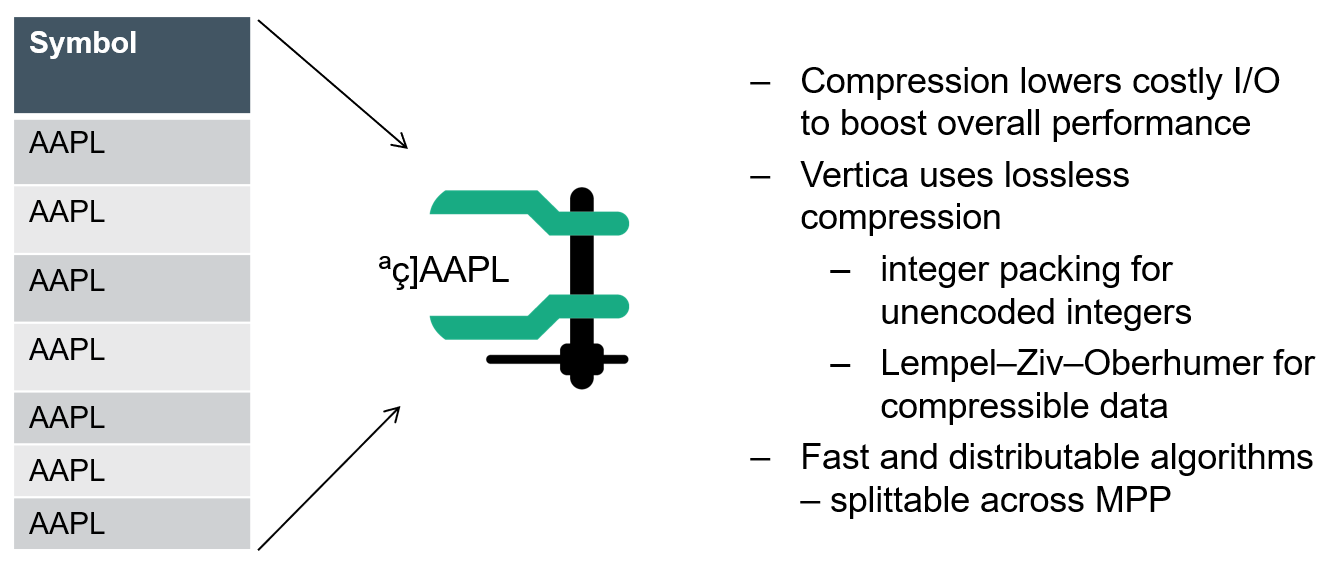
Compression, on the other hand, transforms data into a compact format. Vertica uses several different compression methods and automatically chooses the best one for the data being compressed. Using compression, Vertica stores more data, and uses less hardware than other databases.
In one experiment, a text file containing a million random integers between 1 and 10 million and a size of 7.5 MB was compressed using gzip (sorted and unsorted data) and the size compared to its original version as well as Vertica. The unsorted gzip version averaged the compression ratio of 2.1, sorted version was around 3.3, whereas Vertica managed a respectable 12.5.
In another example, Vertica has a customer that collects metrics from some meters. There are 4 columns in the schema: Metric: There are a few hundred metrics collected. Meter: There are a couple of thousand meters. Collection Time Stamp: Each meter spits out metrics every 5 minutes, 10 minutes, hour, etc., depending on the metric. Metric Value: A 64-bit floating point value. A baseline file of 200 million comma separated values (CSV) of the meter/metric/time/value rows takes 6200 MB, for 32 bytes per row. Compressing with gzip reduces this to 1050 MB. By sorting the data on metric, meter, and collection time, Vertica not only optimises common query predicates (which specify the metric or a time range), but exposes great compression opportunities for each column. The total size for all the columns in Vertica is 418MB (slightly over 2 bytes per row). Metric: There aren’t many. With RLE, it is as if there are only a few hundred rows. Vertica compressed this column to 5 KB. Meter: There are quite a few, and there is one record for each meter for each metric. With RLE, Vertica brings this down to a mere 35 MB. Collection Time Stamp: The regular collection intervals present a great compression opportunity. Vertica compressed this column to 20 MB. Metric Value: Some metrics have trends (like lots of 0 values when nothing happens). Others change gradually with time. Some are much more random, and less compressible. However, Vertica compressed the data to only 363MB.
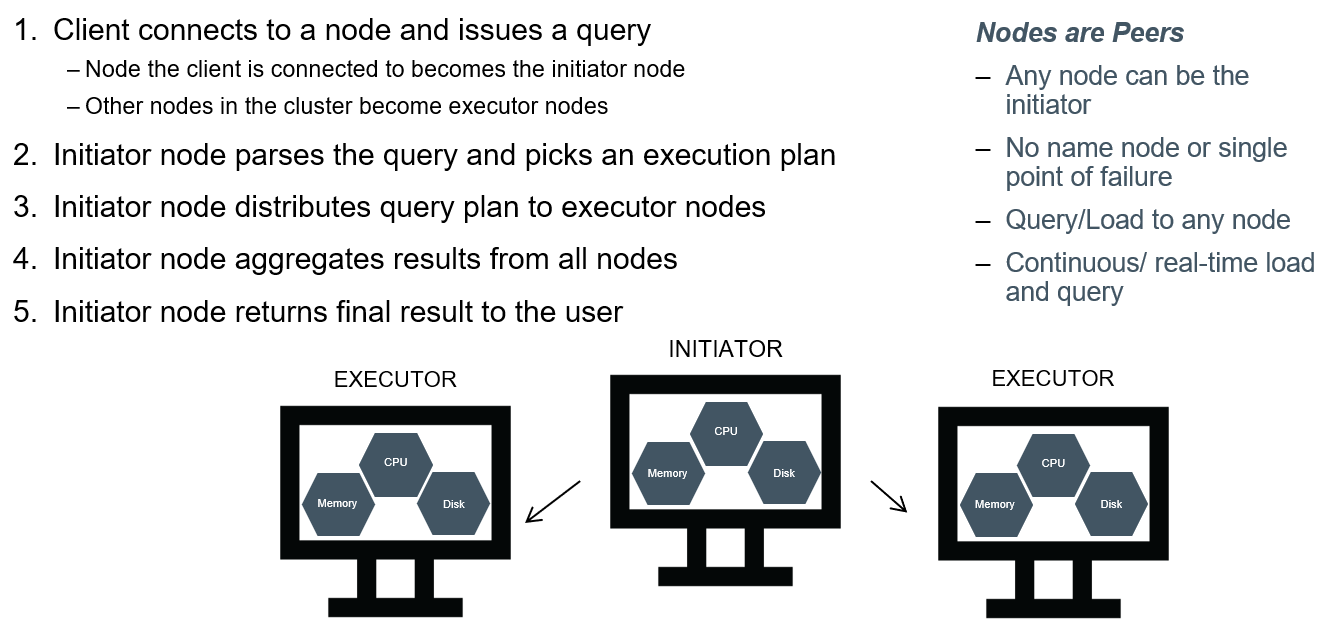
MPP Scale-Out And Distributed Queries
Vertica is not just an analytical database; it is a distributed, ‘shared-nothing’ analytical database capable of running on clusters of inexpensive, off-the-shelf servers, Amazon and Azure Cloud servers, and Hadoop. Its performance can not only be tuned with features like resource pools and projections, but it can be scaled simply by adding new servers to the cluster.
Data within a table may be spread across a Vertica cluster either by replicating the data across all nodes or by ‘segmenting’ the data by attribute values using a consistent hashing schema. This allows many classes of joins to be performed without moving the data across the network. Vertica considers CPU, network and storage access costs when optimising query plans, and parallelizes computation based on SQL’s JOIN keys, GROUP BY keys, and PARTITION BY keys.
Clustering speeds up performance by parallelizing querying and loading across the nodes in the cluster for higher throughput.
Clustering also allows the database to maintain RAID-like high availability in case one or more nodes are down and no longer part of the quorum. This provides a robust mechanism to ensure little to no downtime as multiple copies of same data are stored on different nodes.
The traditional method to ensure that a database system can recover from a crash is to use logging and (in the case of a distributed databases), a protocol called two-phase commit. The main idea is to write in a sequential log a log record for each update operation before the operation is actually applied to the tables on the disk. These log records are a redundant copy of the data in the database, and when a crash occurs, they can be replayed to ensure that transactions are atomic – that is, all of the updates of a transaction appear to have occurred, or none of them do. The two-phase commit protocol is then used to ensure that all of the nodes in a distributed database agree that a transaction has successfully committed; it requires several additional log records to be written. Log-based recovery is widely used in other commercial systems, as it provides strong recoverability guarantees at the expense of significant performance and disk space overhead. Vertica has a unique approach to distributed recoverability that avoids these costs. The basic idea is to exploit the distributed nature of a Vertica database. The Vertica DB Designer ensures that every column in every table in the database is stored on at least k+1 machines in the Vertica cluster. We call such a database k-safe, because if k machines crash or otherwise fail, a complete copy of the database is still available. As long as k or fewer machines fail simultaneously, a crashed machine can recover its state by copying data about transactions that committed or aborted while it was crashed from other machines in the system. This approach does not require logging because nodes replicating the data ensure that a recovering machine always has another (correct) copy of the data to compare against, replacing the role of a log in a traditional database. As long as k-safety holds, there is always one machine that knows the correct outcome (commit or abort) of every transaction. In the unlikely event that the system loses k-safety, Vertica brings the database back to a consistent point in time across all nodes. K-safety also means that Vertica is highly available: it can tolerate the simultaneous crash of up to any k machines in a grid without interrupting query processing. The value of k can be configured to provide the desired trade-off between hardware costs and availability guarantees.
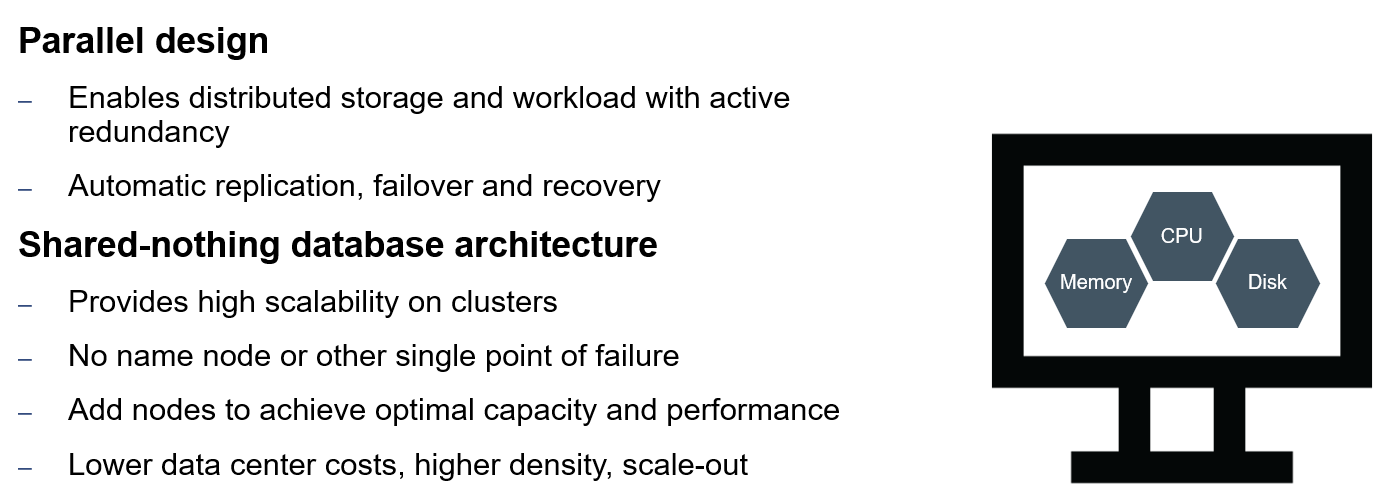
It is instructive to contrast Vertica’s high-availability schemes with traditional database systems where high availability is achieved through the use of active standbys – essentially completely unused hardware that has an exact copy of the database and is ready to take over in the event of a primary database failure. Unlike Vertica’s k-safe design employing different sort orders, active standbys simply add to the cost of the database system without improving performance. Because Vertica is k-safe, it supports hot-swapping of nodes. A node can be removed, and the database will continue to process queries (at a lower rate). Conversely, a node can be added, and the database will automatically allocate a collection of objects to that node so that it can begin processing queries, increasing database performance automatically.
Projections
Projections store data in a format that optimises query execution. Similar to materialised vies, they store results sets on disk rather than compute them each time they are used in a query. Vertica automatically refreshes these result sets with updated or new data.
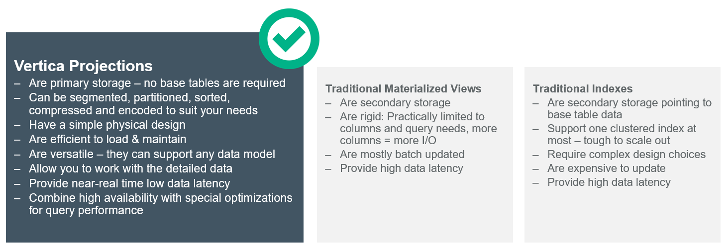
A Vertica table typically has multiple projections, each defined to contain different content. Content for the projections of the given table can differ in scope and how it is organised. These differences can generally be divided into the following projection types:
- Superprojections – a superprojection contains all the column of the table. For each table in the database, Vertica requires a minimum of one superprojection. Under certain conditions, Vertica automatically creates a table’s superprjection immediately on the table creation. Vertica also creates a superprojection when you first load data into that table, if none exists already.
- Query-Specific Projections – A query-specific projection contains only the subset of table columns to process a given query. Query-specific projections significantly improve the performance of those queries for which they are optimised.
- Aggregate Projections – Queries which include expressions or aggregate functions such as SUM and COUNT can perform more efficiently when they use projections that already contain the aggregated data. This is especially true for queries on large values of data.
Projections provide the following benefits:
- Compress and encode data to reduce storage space. Additionally, Vertica operates on the encoded data representation whenever possible to avoid the cost of decoding. This combination of compression and encoding optimises disk space while maximising query performance.
- Facilitate distribution across the database cluster. Depending on their size, projections can be segmented or replicated across cluster nodes. For instance, projections for large tables can be segmented and distributed across all nodes. Unsegmented projections for small tables can be replicated across all nodes.
- Transparent to end-users. The Vertica query optimiser automatically picks up the best projections to execute a given query.
- Provide high-availability and recovery. Vertica duplicates table columns on at least K+1 nodes in the cluster. If one machine fails in a K-Safe environment, the database continues to operate using replicated data on the remaining nodes. When the node resumes normal operation, it automatically queries other nodes to recover data and lost objects.
These architectural differences – column storage, compression, MPP Scale-Out architecture and the ability to distribute a query are what fundamentally enable analytic applications based on Vertica to scale seamlessly and offer many more users access to much more data.
In Part 2 of this series I will dive into installing Vertica on a cluster of inexpensive, desktop-class machines i.e. three Lenovo Tiny units running Ubuntu Server and go over some of the administrative tools e.g. Management Console, metadata queries etc. used to manage it.
http://scuttle.org/bookmarks.php/pass?action=addThis entry was posted on Friday, January 5th, 2018 at 11:44 am and is filed under MPP RDBMS, SQL. You can follow any responses to this entry through the RSS 2.0 feed. You can leave a response, or trackback from your own site.


Hello Kind of what I've been looking for - thanks for posting. I don't use Snowflake but gives me an…