bicortex

Using Python and Tableau to Scrape and Visualize Twitter User Data

March 8th, 2016 / No Comments » / by admin

Note: all the code and additional files for this post can be downloaded from my OneDrive folder HERE.

Introduction

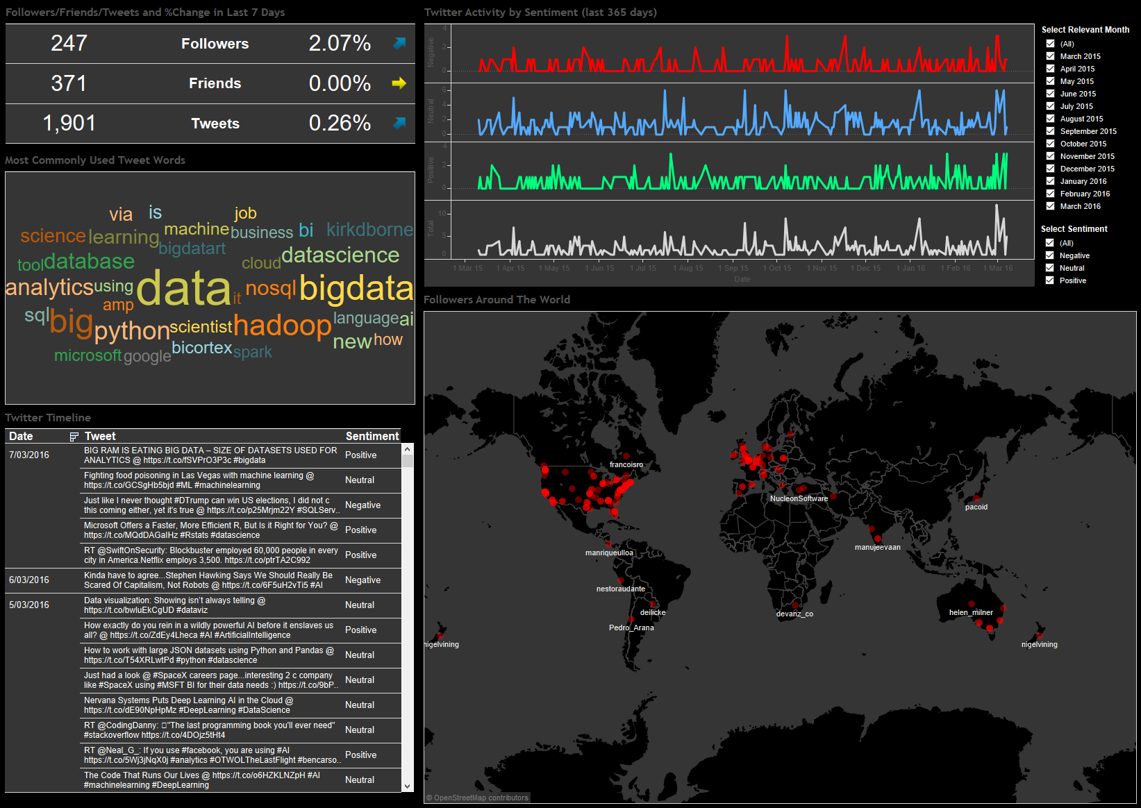
What can I say…I like Twitter and I use it often to get interesting content links on data-related topics and find out what other people I follow are sharing. I covered Twitter-related stuff (sentiment analysis, Twitter timeline harvesting etc.) a number of times in the past, mainly HERE, HERE and HERE but since Twitter data is so rich and easy to work with (their API is pretty straightforward, especially coupled with Python wrappers such as Twython) and I have never gone down the path of visualising my findings I thought it would be a good idea to slap together a simple dashboard depicting some of the scraped data. To make it more fun and to make the dashboard look more polished I also analysed the sentiment of each tweet and geocoded my followers resulting in the Tableau dashboard as per below (click on image to expand).

In order to access Twitter data through a Python script first we will need to register a new Twitter app and download necessary Python libraries (assuming you already have Python installed). Registering the app can be done HERE, where upon filling out some details you should be issued with an API Key (Consumer Key) and API Secret (Consumer Secret). For this demo I will be authenticating into Twitter using OAuth2 i.e. application authentication. With application-only authentication you don’t have the context of an authenticated user and this means that any request to API for endpoints that require user context, such as posting tweets, will not work. However, the set of endpoints that will still be available can have a higher rate limit thus allowing for more frequent querying and data acquisitions (you can find more details on how app authentication works HERE). The API keys are stored in a configuration file, in this case called ‘params.cfg’, which is stored in the same directory as our SQLite database and Python script file. When it comes to Python libraries required, I have chosen the following for this demo, some of which go beyond ‘batteries included’ Python mantra so a quick ‘pip install…’ should do the job:

• Twython – Python wrapper for Twitter API
• Configparser – Python configuration file (storing API Secret and API Key values) parser
• Sqlite3 – relational database for data storage
• Requests – HTTP library (here used for sentiment querying)
• NLTK – natural language/text processing library
• tqdm – terminal progress meter
• Geopy – Python library for popular geocoding services

Python Code

Let’s go through the code (full script as well as all other files can be downloaded from my OneDrive folder HERE) and break it down into logical sections describing different functions. For this demo I wanted my script to do the following:

• Create SQLite database if it does not exist with all the underlying schema for storing user timeline, followers geo-located details and most commonly used words
• Acquire selected user timeline tweets (maximum number allowed by Twitter at this time is 3200) and insert them into the database table
• Assign sentiment value i.e. positive, negative or neutral by querying THIS API (maximum number of API calls allowed is 45,000/month) and update the table storing user timeline tweets with the returned values
• Using NLTK, ‘clean up’ tweets e.g. removing stop words, lemmitize words etc., remove some unwanted characters and hyper links and finally insert the most commonly occurring words into a table
• Acquire user followers’ data and where possible geocode their location using MapQuest API

To do all this, firstly, let’s create our configuration file called ‘params.cfg’ which will store our API keys. Given that most commercially available APIs for sentiment analysis or geocoding are not free or at the very least require you to sign up to make the API key available, this would also be a good place to store those. For this demo we will be using free services so the only values saved in the config file are the secret key and consumer key as per below.

Now we can start building up our script, importing necessary Python modules, declaring variables and their values and referencing our configuration file data as per the snippet below (the highlighted line needs to be populated with the user name referencing the account timeline we’re trying to scrape).

#import relevant libraries and set up variables' values
import twython
import configparser
import sqlite3
import os
import platform
import re
import requests
import sys
from nltk.corpus import stopwords
from nltk.stem import WordNetLemmatizer
from nltk.tokenize import word_tokenize
import time
from collections import Counter
from tqdm import tqdm
from geopy.geocoders import GoogleV3
from geopy.exc import GeocoderQuotaExceeded

MaxTweetsAPI = 3200
StatusesCount = 200
WordCloudTweetNo = 40
IncludeRts = 1
ExcludeReplies = 0
SkipStatus = 1
ScreenName = 'user twitter handle' #e.g. @bicortex
SentimentURL = 'http://text-processing.com/api/sentiment/'
config = configparser.ConfigParser()
config.read('params.cfg')
AppKey = config.get('TwitterAuth','AppKey')
AppSecret = config.get('TwitterAuth','AppSecret')

Next, let’s set up our SQLite database and its schema. Depending on whether I’m at work or using my home computer I tend to move between Windows and Linux so you may want to adjust the first IF/ELSE statement to reflect your environment path and system (highlighted sections).

#Set up database objects' schema
if platform.system() == 'Windows':
    db_location = os.path.normpath('Your_Windows_Directory_Path/twitterDB.db') #e.g. 'C:/Twitter_Scraping_Project/twitterDB.db'
else:
    db_location = r'/Your_Linux_Directory_Path/twitterDB.db' #e.g. '/home/username/Twitter_Scraping_Project/twitterDB.db'

objectsCreate = {'UserTimeline':
                 'CREATE TABLE IF NOT EXISTS UserTimeline ('
                 'user_id int, '
                 'user_name text, '
                 'screen_name  text, '
                 'user_description text, '
                 'user_location text, '
                 'user_url text, '
                 'user_created_datetime text,'
                 'user_language text ,'
                 'user_timezone text, '
                 'user_utc_offset real,'
                 'user_friends_count real,'
                 'user_followers_count real,'
                 'user_statuses_count real,'
                 'tweet_id int,'
                 'tweet_id_str text,'
                 'tweet_text text,'
                 'tweet_created_timestamp text,'
                 'tweet_probability_sentiment_positive real,'
                 'tweet_probability_sentiment_neutral real,'
                 'tweet_probability_sentiment_negative real,'
                 'tweet_sentiment text, '
                 'PRIMARY KEY(tweet_id, user_id))',

                 'FollowersGeoData':
                 'CREATE TABLE IF NOT EXISTS FollowersGeoData ('
                 'follower_id int,'
                 'follower_name text,'
                 'follower_location text,'
                 'location_latitude real,'
                 'location_longitude real,'
                 'PRIMARY KEY (follower_id))',

                 'WordsCount':
                 'CREATE TABLE IF NOT EXISTS WordsCount ('
                 'word text,'
                 'frequency int)'}

#create database file and schema using the scripts above
db_is_new = not os.path.exists(db_location)
with sqlite3.connect(db_location) as conn:
    if db_is_new:
        print("Creating database schema on " + db_location + " database...\n")
        for t in objectsCreate.items():
            try:
                conn.executescript(t[1])
            except sqlite3.OperationalError as e:
                print (e)
                conn.rollback()
                sys.exit(1)
            else:
                conn.commit()
    else:
        print('Database already exists, bailing out...')

UserTimelineIDs = []
cur = 'SELECT DISTINCT tweet_ID from UserTimeline'
data = conn.execute(cur).fetchall()
for u in data:
    UserTimelineIDs.extend(u)

UserFollowerIDs = []
cur = 'SELECT DISTINCT follower_id from FollowersGeoData'
data = conn.execute(cur).fetchall()
for f in data:
    UserFollowerIDs.extend(f)

Next, we will define a simple function to check for Twitter API rate limit. Twitter limits the number of calls we can make to a specific API endpoint e.g. at the time of writing this post user timeline endpoint has a limit of 300 calls in a 15 minutes window when using with the application authentication and 180 calls when used with the user authentication. To allow our script to continue without Twython complaining of us exceeding the allowed threshold we want to make sure that once we reach this rate limit, the script will pause the execution for a predefined amount of time. Twitter’s ‘application/rate_limit_status’ API endpoint provides us with rate limits defined for each endpoint, the remaining number of calls available as well as the expiration time in epoch time. Using those three values we can allow for the script to sleep until the reset windows has been reset and resume scraping without completely stopping the process. Interestingly enough, ‘application/rate_limit_status’ API endpoint is also rate-limited to 180 calls/15 minute window so you will notice ‘appstatus’ variable also keeping this threshold in check.

#check Twitter API calls limit and pause execution to reset the limit if required
def checkRateLimit(limittypecheck):
    appstatus = {'remaining':1}
    while True:
        if appstatus['remaining'] > 0:
            twitter = twython.Twython(AppKey, AppSecret, oauth_version=2)
            ACCESS_TOKEN = twitter.obtain_access_token()
            twitter = twython.Twython(AppKey, access_token=ACCESS_TOKEN)
            status = twitter.get_application_rate_limit_status(resources = ['statuses', 'application', 'followers'])
            appstatus = status['resources']['application']['/application/rate_limit_status']
            if limittypecheck=='usertimeline':
                usertimelinestatus = status['resources']['statuses']['/statuses/user_timeline']
                if usertimelinestatus['remaining'] == 0:
                    wait = max(usertimelinestatus['reset'] - time.time(), 0) + 1  # addding 1 second pad
                    time.sleep(wait)
                else:
                    return
            if limittypecheck=='followers':
                userfollowersstatus = status['resources']['followers']['/followers/list']
                if userfollowersstatus['remaining'] == 0:
                    wait = max(userfollowersstatus['reset'] - time.time(), 0) + 1  # addding 1 second pad
                    time.sleep(wait)
                else:
                    return
        else :
            wait = max(appstatus['reset'] - time.time(), 0) + 1
            time.sleep(wait)

Now that we have the above function in place we can start scraping Twitter feeds for particular user. The below function queries ‘get_user_timeline’ endpoint for a range of timeline attributes, most important being ‘text’ – the actual tweet string. As Twitter returns a single page of data with the number of tweets defined by the ‘StatusesCount’ variable and we require either the total count of tweets or 3200 of them if the user whose timeline we’re querying has posted more than the 3200 statuses rate limit, we will need to implement paging mechanism. By means of using an API parameter called ‘max_id’ which returns the results with an ID less than (that is, older than) or equal to the specified ID we can create a cursor to iterate through multiple pages, eventually getting to the total tweet count or the 3200 rate limit (whichever’s lower). Finally, we insert all tweets and corresponding attributes into the database.

#grab user timeline twitter feed for the profile selected and store them in a table
def getUserTimelineFeeds(StatusesCount, MaxTweetsAPI, ScreenName, IncludeRts, ExcludeReplies, AppKey, AppSecret):
    #Pass Twitter API and database credentials/config parameters
    twitter = twython.Twython(AppKey, AppSecret, oauth_version=2)
    try:
        ACCESS_TOKEN = twitter.obtain_access_token()
    except twython.TwythonAuthError as e:
        print (e)
        sys.exit(1)
    else:
        try:
            twitter = twython.Twython(AppKey, access_token=ACCESS_TOKEN)
            print('Acquiring tweeter feed for user "{0}"...'.format(ScreenName))
            params = {'count': StatusesCount, 'screen_name': ScreenName, 'include_rts': IncludeRts,'exclude_replies': ExcludeReplies}
            AllTweets = []
            checkRateLimit(limittypecheck='usertimeline')
            NewTweets = twitter.get_user_timeline(**params)
            if NewTweets is None:
                print('No user timeline tweets found for "{0}" account, exiting now...'.format(ScreenName))
                sys.exit()
            else:
                ProfileTotalTweets = [tweet['user']['statuses_count'] for tweet in NewTweets][0]
                if ProfileTotalTweets > MaxTweetsAPI:
                    TweetsToProcess = MaxTweetsAPI
                else:
                    TweetsToProcess = ProfileTotalTweets
                oldest = NewTweets[0]['id']
                progressbar = tqdm(total=TweetsToProcess, leave=1)
                while len(NewTweets) > 0:
                    checkRateLimit(limittypecheck='usertimeline')
                    NewTweets = twitter.get_user_timeline(**params, max_id=oldest)
                    AllTweets.extend(NewTweets)
                    oldest = AllTweets[-1]['id'] - 1
                    if len(NewTweets)!=0:
                        progressbar.update(len(NewTweets))
                progressbar.close()

                AllTweets = [tweet for tweet in AllTweets if tweet['id'] not in UserTimelineIDs]
                for tweet in AllTweets:
                    conn.execute("INSERT OR IGNORE INTO UserTimeline "
                     "(user_id,"
                     "user_name,"
                     "screen_name,"
                     "user_description,"
                     "user_location,"
                     "user_url,"
                     "user_created_datetime,"
                     "user_language,"
                     "user_timezone,"
                     "user_utc_offset,"
                     "user_friends_count,"
                     "user_followers_count,"
                     "user_statuses_count,"
                     "tweet_id,"
                     "tweet_id_str,"
                     "tweet_text,"
                     "tweet_created_timestamp) VALUES (?,?,?,?,?,?,?,?,?,?,?,?,?,?,?,?,?)",(
                    tweet['user']['id'],
                    tweet['user']['name'],
                    tweet['user']['screen_name'],
                    tweet['user']['description'],
                    tweet['user']['location'],
                    tweet['user']['url'],
                    time.strftime('%Y-%m-%d %H:%M:%S', time.strptime(tweet['user']['created_at'],'%a %b %d %H:%M:%S +0000 %Y')),
                    tweet['user']['lang'],
                    tweet['user']['time_zone'],
                    tweet['user']['utc_offset'],
                    tweet['user']['friends_count'],
                    tweet['user']['followers_count'],
                    tweet['user']['statuses_count'],
                    tweet['id'],
                    tweet['id_str'],
                    str(tweet['text'].replace("\n","")),
                    time.strftime('%Y-%m-%d %H:%M:%S', time.strptime(tweet['created_at'],'%a %b %d %H:%M:%S +0000 %Y'))))
                conn.commit()
        except Exception as e:
            print(e)
            sys.exit(1)

Great! Now that we have the user timeline table populated we can proceed with assigning sentiment to each individual record. I used a free service which allows for 45,000 API calls a month. Since there are no batch POST requests available and every single record has to be queried individually we also exclude the ones which have already been assigned the sentiment. Also, the function below takes care of removing certain characters and hyper links as these can interfere with the classification process.

#assign sentiment to individual tweets
def getSentiment(SentimentURL):
        cur = ''' SELECT tweet_id, tweet_text, count(*) as NoSentimentRecCount
                  FROM UserTimeline
                  WHERE tweet_sentiment IS NULL
                  GROUP BY tweet_id, tweet_text '''
        data = conn.execute(cur).fetchone()
        if data is None:
            print('Sentiment already assigned to relevant records or table is empty, bailing out...')
        else:
            print('Assigning sentiment to selected tweets...')
            data = conn.execute(cur)
            payload = {'text':'tweet'}
            for t in tqdm(data.fetchall(),leave=1):
                id = t[0]
                payload['text'] = t[1]
                #concatnate if tweet is on multiple lines
                payload['text'] = str(payload['text'].replace("\n", ""))
                #remove http:// URL shortening links
                payload['text'] = re.sub(r'http://[\w.]+/+[\w.]+', "", payload['text'], re.IGNORECASE)
                #remove https:// URL shortening links
                payload['text'] = re.sub(r'https://[\w.]+/+[\w.]+', "", payload['text'], re.IGNORECASE)
                #remove certain characters
                payload['text'] = re.sub('[@#\[\]\'"$.;{}~`<>:%&^*()-?_!,+=]', "", payload['text'])
                #print(payload['text'])
                try:
                    post=requests.post(SentimentURL, data=payload)
                    response = post.json()
                    conn.execute("UPDATE UserTimeline "
                                    "SET tweet_probability_sentiment_positive = ?, "
                                    "tweet_probability_sentiment_neutral = ?, "
                                    "tweet_probability_sentiment_negative = ?, "
                                    "tweet_sentiment = ? WHERE tweet_id = ?",
                                    (response['probability']['neg'],
                                    response['probability']['neutral'],
                                    response['probability']['pos'],
                                    response['label'], id))
                    conn.commit()
                except Exception as e:
                    print (e)
                    sys.exit(1)

Next, we can look at the word count function. This code takes advantage of the NLTK library to tokenize the tweets, remove certain stop words, lemmatize the tweets, remove unwanted characters and finally work out the top counts for individual words. The output gets inserted into the separate table in the same database simply as the top occurring word and frequency attributes.

#get most commonly occurring (40) words in all stored tweets
def getWordCounts(WordCloudTweetNo):
    print('Fetching the most commonly used {0} words in the "{1}" feed...'.format(WordCloudTweetNo, ScreenName))
    cur = "DELETE FROM WordsCount;"
    conn.execute(cur)
    conn.commit()
    cur = 'SELECT tweet_text FROM UserTimeline'
    data = conn.execute(cur)
    StopList = stopwords.words('english')
    Lem = WordNetLemmatizer()
    AllWords = ''
    for w in tqdm(data.fetchall(),leave=1):
            try:
                #remove certain characters and strings
                CleanWordList = re.sub(r'http://[\w.]+/+[\w.]+', "", w[0], re.IGNORECASE)
                CleanWordList = re.sub(r'https://[\w.]+/+[\w.]+', "", CleanWordList, re.IGNORECASE)
                CleanWordList = re.sub(r'[@#\[\]\'"$.;{}~`<>:%&^*()-?_!,+=]', "", CleanWordList)
                #tokenize and convert to lower case
                CleanWordList = [words.lower() for words in word_tokenize(CleanWordList) if words not in StopList]
                #lemmatize words
                CleanWordList = [Lem.lemmatize(word) for word in CleanWordList]
                #join words
                CleanWordList =' '.join(CleanWordList)
                AllWords += CleanWordList
            except Exception as e:
                print (e)
                sys.exit(e)
    if AllWords is not None:
        words = [word for word in AllWords.split()]
        c = Counter(words)
        for word, count in c.most_common(WordCloudTweetNo):
            conn.execute("INSERT INTO WordsCount (word, frequency) VALUES (?,?)", (word, count))
            conn.commit()

Next, we will source the data on the user’s followers, again using the cursor to iterate through each page (excluding the ones who did not list their location), insert it into the database and finally geo-code their location using Google API which will attempt assigning latitude and longitude values where possible and update the database table accordingly. Caution though, since Google Geo API is limited to processing 2500 calls free of charge, if you have run up more than this limit of geo-located followers you may either want to pay to have this limit expanded or geocode the data in daily batches.

#geocode followers where geolocation data stored as part of followers' profiles
def GetFollowersGeoData(StatusesCount, ScreenName, SkipStatus, AppKey, AppSecret):
    print('Acquiring followers for Twitter handle "{0}"...'.format(ScreenName))
    twitter = twython.Twython(AppKey, AppSecret, oauth_version=2)
    ACCESS_TOKEN = twitter.obtain_access_token()
    twitter = twython.Twython(AppKey, access_token=ACCESS_TOKEN)
    params = {'count': StatusesCount, 'screen_name': ScreenName, 'skip_status':1}
    checkRateLimit(limittypecheck='usertimeline')
    TotalFollowersCount = twitter.get_user_timeline(**params)
    TotalFollowersCount = [tweet['user']['followers_count'] for tweet in TotalFollowersCount][0]

    progressbar=tqdm(total=TotalFollowersCount, leave=1)
    Cursor = -1
    while Cursor != 0:
        checkRateLimit(limittypecheck='followers')
        NewGeoEnabledUsers = twitter.get_followers_list(**params, cursor=Cursor)
        Cursor = NewGeoEnabledUsers['next_cursor']
        progressbar.update(len(NewGeoEnabledUsers['users']))
        NewGeoEnabledUsers = [[user['id'], user['screen_name'], user['location']] for user in NewGeoEnabledUsers['users'] if user['location'] != '']
        #AllGeoEnabledUsers.extend(NewGeoEnabledUsers)
        for user in NewGeoEnabledUsers:
            if user[0] not in UserFollowerIDs:
                conn.execute("INSERT OR IGNORE INTO FollowersGeoData ("
                             "follower_id,"
                             "follower_name,"
                             "follower_location)"
                             "VALUES (?,?,?)",
                            (user[0], user[1], user[2]))
                conn.commit()
    progressbar.close()
    print('')
    print('Geo-coding followers location where location variable provided in the user profile...')
    geo = GoogleV3(timeout=5)
    cur = 'SELECT follower_id, follower_location FROM FollowersGeoData WHERE location_latitude IS NULL OR location_longitude IS NULL'
    data = conn.execute(cur)
    for location in tqdm(data.fetchall(), leave=1):
        try:
            try:
                followerid = location[0]
                #print(location[1])
                geoparams = geo.geocode(location[1])
            except GeocoderQuotaExceeded as e:
                print(e)
                return
                #print(geoparams)
            else:
                if geoparams is None:
                    pass
                else:
                    latitude = geoparams.latitude
                    longitude = geoparams.longitude
                    conn.execute("UPDATE FollowersGeoData "
                                "SET location_latitude = ?,"
                                "location_longitude = ?"
                                "WHERE follower_id = ?",
                                (latitude,longitude,followerid))
                    conn.commit()
        except Exception as e:
            print("Error: geocode failed on input %s with message %s"%(location[2], e))
            continue

Finally, running the ‘main’ function will execute the above in a sequential order, displaying progress bar for all API related calls as per below.

#run all functions
def main():
    getUserTimelineFeeds(StatusesCount, MaxTweetsAPI, ScreenName, IncludeRts, ExcludeReplies, AppKey, AppSecret)
    getSentiment(SentimentURL)
    getWordCounts(WordCloudTweetNo)
    GetFollowersGeoData(StatusesCount, ScreenName, SkipStatus, AppKey, AppSecret)
    conn.close()

if __name__ == "__main__":
    main()

Visualizing Data in Tableau

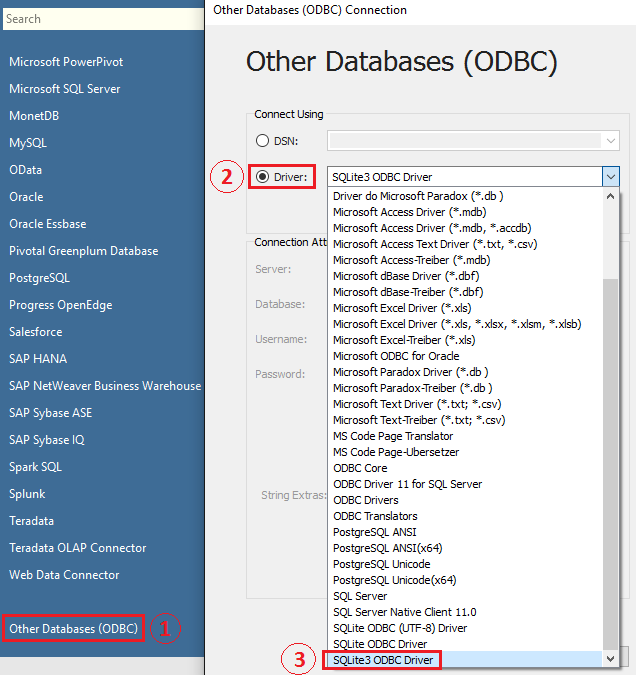
Now that we have our three database tables populated, let create a simple dashboard in Tableau. Since we implemented our data storage layer in SQLite, first we need to download SQLite driver to enable it to talk to Tableau. Once installed (I downloaded mine from HERE), you should able to select it from options available under ‘Other Databases (ODBC)’ data sources.

Once the connection has been established we can finally commence building out our dashboard but before we begin, a quick word of caution – if you want to turn this demo into a more robust solution, SQLite database back-end, even though good enough for this proof of concept, may not play well with Tableau. I came across a few issues with data types support and since SQLite has not been designed with a server/client architecture in mind, chances are that Tableau has a better out-of-the-box compatibility when coupled with RDBMSs which it natively supports e.g. MySQL, PostgeSQL, MSSQL etc. Below is a notification pop-up warning of the lack of support for some features when using SQLite ODBC connection.

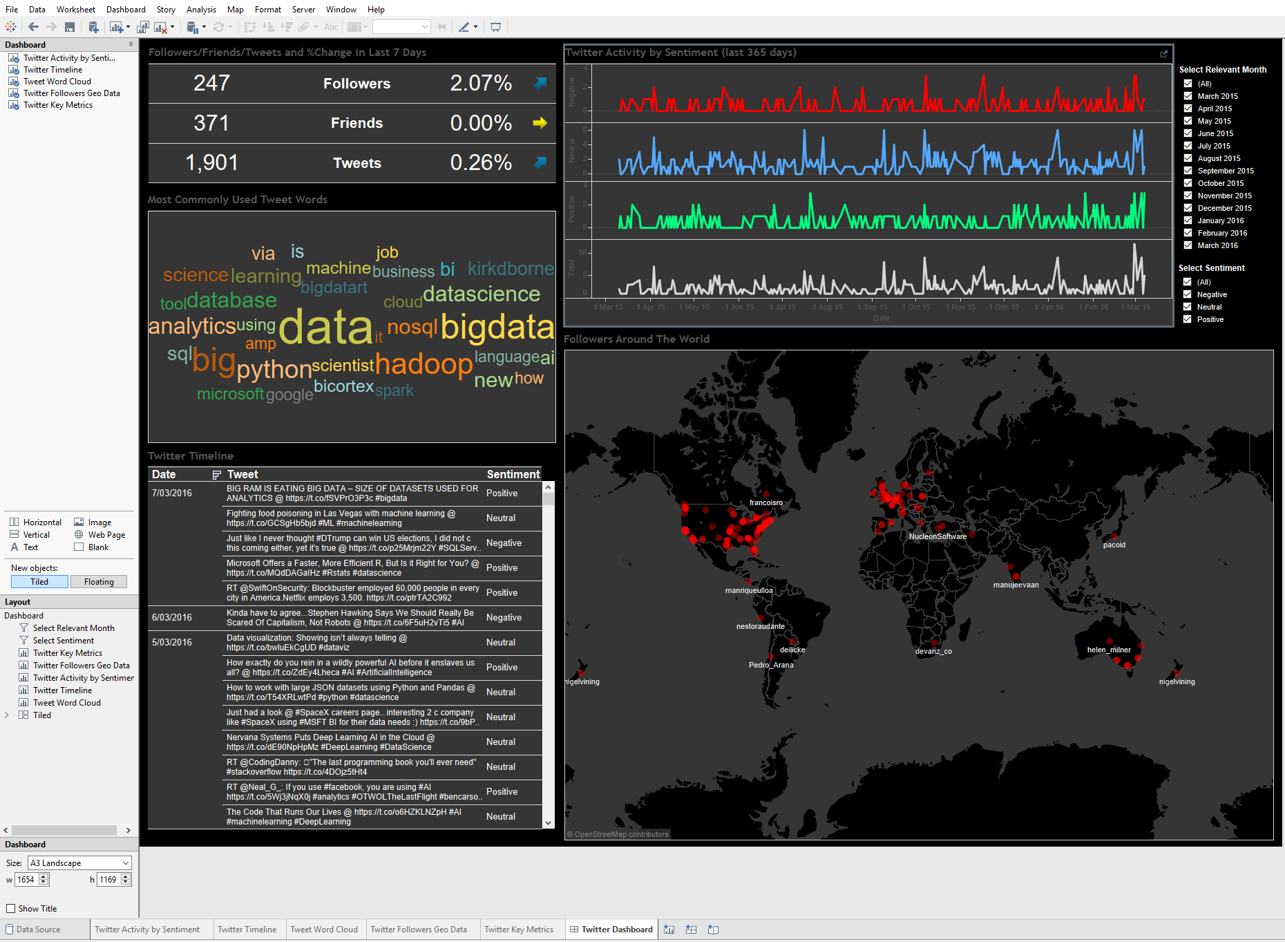
Continuing on, in Tableau, I have created four different sheets, two of them pointing to the same data source (as they rely on the same UserTimeline table) and the remaining two pointing to two other tables i.e. WordsCount and FollowersGeoData. The SQL queries used are mostly just straightforward SELECT statements out of their respective tables, with the one driving followers/tweets/friends counts structured to account for changes captured in the last seven days as per the code below.

SELECT
friends_count as counts,
((friends_count - last_weeks_friends_count)/last_weeks_friends_count)  as percentage_change, 'Friends' as category
FROM
(SELECT 
MAX(user_friends_count) as friends_count,
MAX(user_followers_count) as followers_count,
MAX(user_statuses_count) as statuses_count,
(SELECT user_friends_count FROM UserTimeLine
		WHERE tweet_created_timestamp < date('now','-7 days')
		ORDER BY ROWID ASC LIMIT 1
) as last_weeks_friends_count,
(SELECT user_followers_count FROM UserTimeLine
		WHERE tweet_created_timestamp < date('now','-7 days')
		ORDER BY ROWID ASC LIMIT 1
) as last_weeks_followers_count,
(SELECT user_statuses_count FROM UserTimeLine
		WHERE tweet_created_timestamp < date('now','-7 days')
		ORDER BY ROWID ASC LIMIT 1
) as last_weeks_statuses_count
FROM UserTimeLine) 
UNION ALL
SELECT
followers_count as counts,
((followers_count - last_weeks_followers_count)/last_weeks_followers_count) as percentage_change, 'Followers' as category
FROM
(SELECT 
MAX(user_friends_count) as friends_count,
MAX(user_followers_count) as followers_count,
MAX(user_statuses_count) as statuses_count,
(SELECT user_friends_count FROM UserTimeLine
		WHERE tweet_created_timestamp < date('now','-7 days')
		ORDER BY ROWID ASC LIMIT 1
) as last_weeks_friends_count,
(SELECT user_followers_count FROM UserTimeLine
		WHERE tweet_created_timestamp < date('now','-7 days')
		ORDER BY ROWID ASC LIMIT 1
) as last_weeks_followers_count,
(SELECT user_statuses_count FROM UserTimeLine
		WHERE tweet_created_timestamp < date('now','-7 days')
		ORDER BY ROWID ASC LIMIT 1
) as last_weeks_statuses_count
FROM UserTimeLine) UNION ALL
SELECT
statuses_count as counts,
((statuses_count - last_weeks_statuses_count)/last_weeks_statuses_count)  as percentage_change, 'Tweets' as category
FROM
(SELECT 
MAX(user_friends_count) as friends_count,
MAX(user_followers_count) as followers_count,
MAX(user_statuses_count) as statuses_count,
(SELECT user_friends_count FROM UserTimeLine
		WHERE tweet_created_timestamp < date('now','-7 days')
		ORDER BY ROWID ASC LIMIT 1
) as last_weeks_friends_count,
(SELECT user_followers_count FROM UserTimeLine
		WHERE tweet_created_timestamp < date('now','-7 days')
		ORDER BY ROWID ASC LIMIT 1
) as last_weeks_followers_count,
(SELECT user_statuses_count FROM UserTimeLine
		WHERE tweet_created_timestamp < date('now','-7 days')
		ORDER BY ROWID ASC LIMIT 1
) as last_weeks_statuses_count
FROM UserTimeLine)

All there is left to do is to position each sheets’ visualisation on the dashboard and vuala…the complete dashboard looks like this (click on image to expand).

Again, all the code, database and Tableau solution files can be downloaded from my OneDrive folder HERE. Since I have removed the database connection details from all data sources, if you’re thinking of replicating this solution on your own machine, all you need to do is point each data source to SQLite database location as per the video below.

Posted in: Programming, SQL, Tableau

Tags: Programming, Python, Social Networks, SQL, Tableau

Microsoft Azure SQL Data Warehouse Quick Review and Amazon Redshift Comparison – Part 2

January 15th, 2016 / 4 Comments » / by admin

In the first part of this series I briefly explored Microsoft Azure Data Warehouse key differentiating features that set it apart from the likes of AWS Redshift and outlined how we can load the Azure DW with sample TICKIT database data. In this final post I will go over some of the findings from comparing query execution speed across AWS/Azure DW offerings and briefly look at the reporting/analytics status quo.

My test ‘hardware’ set-up composition was characterized by the following specifications where, as mentioned in PART ONE, Amazon seems to adopt a bit less of a cloak-and-dagger approach.

Graphing the results, I assigned the following monikers to each environment based on its specifications/price point.

• Azure SQL DW 100 DWU – Azure Data Warehouse 100 Data Warehouse Units
• Azure SQL DW 500 DWU – Azure Data Warehouse 500 Data Warehouse Units
• Azure SQL DW 1000 DWU – Azure Data Warehouse 1000 Data Warehouse Units
• Azure SQL DW 2000 DWU – Azure Data Warehouse 2000 Data Warehouse Units
• Redshift 3 x dc1.large – AWS Redshift 3 x large dense compute nodes
• Redshift 2 x dc1.8xlarge – AWS Redshift 2 x extra-large dense compute nodes

Testing Methodology and Configuration Provisions

Each table created on Azure DW also had clustered columnstore index created on it, which as of December 2015, is a default behaviour when issuing a CREATE TABLE DDL statement unless specified otherwise i.e. using a HEAP option with the table creation statement. Clustered columnstore indexes provide better performance and data compression than a heap or rowstore clustered index. Also, each fact table and its data created in Azure DW was distributed using hashing values on identity fields e.g. Sales table –> saleid column, Listing table –> listid column, whereas a round-robin algorithm was used for dimension tables data distribution. A hash distributed table is a table whose rows are dispersed across multiple distributions based on a hash function applied to a column. When processing queries involving distributed tables, SQL DW instances execute multiple internal queries, in parallel, within each SQL instance, one per distribution.  These separate processes (independent internal SQL queries) are executed to handle different distributions during query and load processing. A round-robin distributed table is a table where the data is evenly (or as evenly as possible) distributed among all the distributions. Buffers containing rows of data are allocated in turn (hence the name round robin) to each distribution. The process is repeated until all data buffers have been allocated. At no stage is the data sorted or ordered in a round robin distributed table. A round robin distribution is sometimes called a random hash for this reason.

Each table on AMS Redshift database was assigned a distkey and a sortkey which are a powerful set of tools for optimizing query performance. A table’s distkey is the column on which it’s distributed to each node. Rows with the same value in this column are guaranteed to be on the same node. The goal in selecting a table distribution style is to minimize the impact of the redistribution step by locating the data where it needs to be before the query is executed. A table’s sortkey is the column by which it’s sorted within each node. The Amazon Redshift query optimizer uses sort order when it determines optimal query plans.

The following allocation was made for each table in the TICKIT database schema on AWS Redshift database.

On Azure Data Warehouse, after populating TICKIT schema and before running all queries, clustered columnstore indexes were created on each table. Also, at a minimum, Microsoft recommends creating at least single-column statistics on every column on every table which in case of SQL Data Warehouse are user-defined i.e. need to be created manually and managed manually. As SQL Data Warehouse does not have a system stored procedure equivalent to ‘sp_create_stats’ in SQL Server, the following stored procedure was used to create a single column statistics object on every column of the database that didn’t already one, with FULLSCAN option defined for @create_type.

CREATE PROCEDURE    [dbo].[prc_sqldw_create_stats]
(   @create_type    tinyint -- 1 default 2 Fullscan 3 Sample
,   @sample_pct     tinyint
)
AS

IF @create_type NOT IN (1,2,3)
BEGIN
    THROW 151000,'Invalid value for @stats_type parameter. Valid range 1 (default), 2 (fullscan) or 3 (sample).',1;
END;

IF @sample_pct IS NULL
BEGIN;
    SET @sample_pct = 20;
END;

IF OBJECT_ID('tempdb..#stats_ddl') IS NOT NULL
BEGIN;
    DROP TABLE #stats_ddl;
END;

CREATE TABLE #stats_ddl
WITH    (   DISTRIBUTION    = HASH([seq_nmbr])
        ,   LOCATION        = USER_DB
        )
AS
WITH T
AS
(
SELECT      t.[name]                        AS [table_name]
,           s.[name]                        AS [table_schema_name]
,           c.[name]                        AS [column_name]
,           c.[column_id]                   AS [column_id]
,           t.[object_id]                   AS [object_id]
,           ROW_NUMBER()
            OVER(ORDER BY (SELECT NULL))    AS [seq_nmbr]
FROM        sys.[tables] t
JOIN        sys.[schemas] s         ON  t.[schema_id]       = s.[schema_id]
JOIN        sys.[columns] c         ON  t.[object_id]       = c.[object_id]
LEFT JOIN   sys.[stats_columns] l   ON  l.[object_id]       = c.[object_id]
                                    AND l.[column_id]       = c.[column_id]
                                    AND l.[stats_column_id] = 1
LEFT JOIN   sys.[external_tables] e ON  e.[object_id]       = t.[object_id]
WHERE       l.[object_id] IS NULL
AND         e.[object_id] IS NULL -- not an external table
)
SELECT  [table_schema_name]
,       [table_name]
,       [column_name]
,       [column_id]
,       [object_id]
,       [seq_nmbr]
,       CASE @create_type
        WHEN 1
        THEN    CAST('CREATE STATISTICS '+QUOTENAME('stat_'+table_schema_name+ '_' + table_name + '_'+column_name)+' ON '+QUOTENAME(table_schema_name)+'.'+QUOTENAME(table_name)+'('+QUOTENAME(column_name)+')' AS VARCHAR(8000))
        WHEN 2
        THEN    CAST('CREATE STATISTICS '+QUOTENAME('stat_'+table_schema_name+ '_' + table_name + '_'+column_name)+' ON '+QUOTENAME(table_schema_name)+'.'+QUOTENAME(table_name)+'('+QUOTENAME(column_name)+') WITH FULLSCAN' AS VARCHAR(8000))
        WHEN 3
        THEN    CAST('CREATE STATISTICS '+QUOTENAME('stat_'+table_schema_name+ '_' + table_name + '_'+column_name)+' ON '+QUOTENAME(table_schema_name)+'.'+QUOTENAME(table_name)+'('+QUOTENAME(column_name)+') WITH SAMPLE '+@sample_pct+'PERCENT' AS VARCHAR(8000))
        END AS create_stat_ddl
FROM T
;

DECLARE @i INT              = 1
,       @t INT              = (SELECT COUNT(*) FROM #stats_ddl)
,       @s NVARCHAR(4000)   = N''
;

WHILE @i <= @t
BEGIN
    SET @s=(SELECT create_stat_ddl FROM #stats_ddl WHERE seq_nmbr = @i);

    PRINT @s
    EXEC sp_executesql @s
    SET @i+=1;
END

DROP TABLE #stats_ddl;

AWS Redshift database, on the other hand, was issued a VACUUM REINDEX command for each table in the TICKIT database in order to analyse the distribution of the values in interleaved sort key columns, reclaims disk space and resorts all rows. Amazon recommends running ANALYZE command alongside the VACUUM statement whenever a significant number of rows is added, deleted or modified to update the statistics metadata, however, given that COPY command automatically updates statistics after loading an empty table, the statistics should already be up-to-date.

Disclaimer

Please note that beyond the measures outlined above, no tuning, tweaking or any other optimization techniques were employed when making this comparison, therefore, the results are only indicative of the performance level in the context of the same data and configuration used. Also, all tests were run when Microsoft Azure SQL Data Warehouse was still in preview hence it is possible that most of the service performance deficiencies or alternatively performance-to-price ratio have now been rectified/improved thus subsequently altering the value proposition if implemented today. Finally, all queries executed in this comparison do not reflect any specific business questions, therefore all SQL statements have a very arbitrary structure and have been assembled to only test computational performance of each service. As such, they do not represent any typical business cases and can only be viewed as a rudimentary performance testing tool.

Test Results

When comparing execution speeds on the same data between those two different services only similar instance classes should be stacked up against each other (typically based on hardware specifications). Given the sometimes ambiguous and deceptive nature of the cloud and its providers’ statements regarding the actual hardware selection/implementation, in this case it is only fair to match them based on the actual service price points. As such, when analysing the results, I excluded Azure SQL Data Warehouse 500 DTU and Azure SQL Data Warehouse 2000 DTU instances (displayed for reference only) and focused on AWS Redshift similarly priced Azure SQL Data Warehouse 100 DTU and Azure SQL Data Warehouse 1000 DTU instances. Also, storage and network transfer fees were not taken into consideration when matching up the price points as these were negligible with the amount of data I used in my case.

All SQL queries run to collect execution times (expressed in seconds) as well as graphical representation of their duration are as per below.

--QUERY 1
SELECT  COUNT(*)
FROM    ( SELECT    COUNT(*) AS counts ,
                    salesid ,
                    listid ,
                    sellerid ,
                    buyerid ,
                    eventid ,
                    dateid ,
                    qtysold ,
                    pricepaid ,
                    commission ,
                    saletime
          FROM      sales
          GROUP BY  salesid ,
                    listid ,
                    sellerid ,
                    buyerid ,
                    eventid ,
                    dateid ,
                    qtysold ,
                    pricepaid ,
                    commission ,
                    saletime
        ) sub;

--QUERY 2
WITH    cte
          AS ( SELECT   SUM(s.pricepaid) AS pricepaid ,
                        sub.* ,
                        u1.email ,
                        DENSE_RANK() OVER ( PARTITION BY sub.totalprice ORDER BY d.caldate DESC ) AS daterank
               FROM     sales s
                        JOIN ( SELECT   l.totalprice ,
                                        l.listid ,
                                        v.venuecity ,
                                        c.catdesc
                               FROM     listing l
                                        LEFT JOIN event e ON l.eventid = e.eventid
                                        INNER JOIN category c ON e.catid = c.catid
                                        INNER JOIN venue v ON e.venueid = v.venueid
                               GROUP BY v.venuecity ,
                                        c.catdesc ,
                                        l.listid ,
                                        l.totalprice
                             ) sub ON s.listid = sub.listid
                        LEFT JOIN users u1 ON s.buyerid = u1.userid
                        LEFT JOIN Date d ON d.dateid = s.dateid
               GROUP BY sub.totalprice ,
                        sub.listid ,
                        sub.venuecity ,
                        sub.catdesc ,
                        u1.email ,
                        d.caldate
             )
    SELECT  COUNT(*)
    FROM    cte;

--QUERY 3
SELECT  COUNT(*)
FROM    ( SELECT    s.* ,
                    u.*
          FROM      sales s
                    LEFT JOIN event e ON s.eventid = e.eventid
                    LEFT JOIN date d ON d.dateid = s.dateid
                    LEFT JOIN users u ON u.userid = s.buyerid
                    LEFT JOIN listing l ON l.listid = s.listid
                    LEFT JOIN category c ON c.catid = e.catid
                    LEFT JOIN venue v ON v.venueid = e.venueid
          INTERSECT
          SELECT    s.* ,
                    u.*
          FROM      sales s
                    LEFT JOIN event e ON s.eventid = e.eventid
                    LEFT JOIN date d ON d.dateid = s.dateid
                    LEFT JOIN users u ON u.userid = s.buyerid
                    LEFT JOIN listing l ON l.listid = s.listid
                    LEFT JOIN category c ON c.catid = e.catid
                    LEFT JOIN venue v ON v.venueid = e.venueid
          WHERE     d.holiday = 0
        ) sub;

--QUERY 4
SELECT  COUNT(*)
FROM    ( SELECT    SUM(sub1.pricepaid) AS price_paid ,
                    sub1.caldate AS date ,
                    sub1.username
          FROM      ( SELECT    s.pricepaid ,
                                d.caldate ,
                                u.username
                      FROM      Sales s
                                LEFT JOIN date d ON s.dateid = s.dateid
                                LEFT JOIN users u ON s.buyerid = u.userid
                      WHERE     s.saletime BETWEEN '2008-12-01' AND '2008-12-31'
                    ) sub1
          GROUP BY  sub1.caldate ,
                    sub1.username
        ) AS sub2;

--QUERY 5
WITH    CTE1 ( c1 )
          AS ( SELECT   COUNT(1) AS c1
               FROM     Sales s
               WHERE    saletime BETWEEN '2008-12-01' AND '2008-12-31'
               GROUP BY salesid
               HAVING   COUNT(*) = 1
             ),
        CTE2 ( c2 )
          AS ( SELECT   COUNT(1) AS c2
               FROM     Listing e
               WHERE    listtime BETWEEN '2008-12-01' AND '2008-12-31'
               GROUP BY listid
               HAVING   COUNT(*) = 1
             ),
        CTE3 ( c3 )
          AS ( SELECT   COUNT(1) AS c3
               FROM     Date d
               GROUP BY dateid
               HAVING   COUNT(*) = 1
             )
    SELECT  COUNT(*)
    FROM    CTE1
            RIGHT JOIN CTE2 ON CTE1.c1 <> CTE2.c2
            RIGHT JOIN CTE3 ON CTE3.c3 = CTE2.c2
                               AND CTE3.c3 <> CTE1.c1
    GROUP BY CTE1.c1
    HAVING  COUNT(*) > 1;

--QUERY 6
WITH    cte
          AS ( SELECT   s1.* ,
                        COALESCE(u.likesports, u.liketheatre, u.likeconcerts,
                                 u.likejazz, u.likeclassical, u.likeopera,
                                 u.likerock, u.likevegas, u.likebroadway,
                                 u.likemusicals) AS interests
               FROM     sales s1
                        LEFT JOIN users u ON s1.buyerid = u.userid
               WHERE    EXISTS ( SELECT s2.*
                                 FROM   sales s2
                                        LEFT JOIN event e ON s2.eventid = e.eventid
                                        LEFT JOIN date d ON d.dateid = s2.dateid
                                        LEFT JOIN listing l ON l.listid = s2.listid
                                                              AND s1.salesid = s2.salesid )
                        AND NOT EXISTS ( SELECT s3.*
                                         FROM   sales s3
                                                LEFT JOIN event e ON s3.eventid = e.eventid
                                                LEFT JOIN category c ON c.catid = e.catid
                                         WHERE  c.catdesc = 'National Basketball Association'
                                                AND s1.salesid = s3.salesid )
             )
    SELECT  COUNT(*)
    FROM    cte
    WHERE   cte.dateid IN (
            SELECT  dateid
            FROM    ( SELECT    ss.dateid ,
                                ss.buyerid ,
                                RANK() OVER ( PARTITION BY ss.dateid ORDER BY ss.saletime DESC ) AS daterank
                      FROM      sales ss
                    ) sub
            WHERE   sub.daterank = 1 );

--QUERY 7
WITH    Temp ( sum_pricepaid, sum_commission, sum_qtysold, eventname, caldate, username, Row1 )
          AS ( SELECT   SUM(s.pricepaid) AS sum_pricepaid ,
                        SUM(s.commission) AS sum_commission ,
                        SUM(s.qtysold) AS sum_qtysold ,
                        e.eventname ,
                        d.caldate ,
                        u.username ,
                        ROW_NUMBER() OVER ( PARTITION BY e.eventname ORDER BY e.starttime DESC ) AS Row1
               FROM     Sales s
                        JOIN Event e ON s.eventid = e.eventid
                        JOIN Date d ON s.dateid = d.dateid
                        JOIN Listing l ON l.listid = s.listid
                        JOIN Users u ON l.sellerid = u.userid
               WHERE    d.holiday <> 1
               GROUP BY e.eventname ,
                        d.caldate ,
                        e.starttime ,
                        u.username
             )
    SELECT  COUNT(*)
    FROM    Temp
    WHERE   Row1 = 1;

--QUERY 8
SELECT  COUNT(*)
FROM    ( SELECT    a.pricepaid ,
                    a.eventname ,
                    NTILE(10) OVER ( ORDER BY a.pricepaid DESC ) AS ntile_pricepaid ,
                    a.qtysold ,
                    NTILE(10) OVER ( ORDER BY a.qtysold DESC ) AS ntile_qtsold ,
                    a.commission ,
                    NTILE(10) OVER ( ORDER BY a.commission DESC ) AS ntile_commission
          FROM      ( SELECT    SUM(pricepaid) AS pricepaid ,
                                SUM(qtysold) AS qtysold ,
                                SUM(commission) AS commission ,
                                e.eventname
                      FROM      Sales s
                                JOIN Date d ON s.dateid = s.dateid
                                JOIN Event e ON s.eventid = e.eventid
                                JOIN Listing l ON l.listid = s.listid
                      WHERE     d.caldate > l.listtime
                      GROUP BY  e.eventname
                    ) a
        ) z;

Even taking Azure SQL DW 500 DWU and Azure SQL DW 2000 DWU out of equation, at face value, it is easy to conclude that Amazon Redshift MPP performed much better across most queries. With the exception of query 8, where Azure SQL DW came out performing a lot better Redshift, Azure SQL DW took a lot longer to compute the results, in some instances 40 times slower then cooperatively priced Redshift instance e.g. query 2. The very last query results, however, show Azure SQL DW performing considerably better in comparison to Redshift, with Amazon’s service also having troubles executing query 6 (hence the lack of results for this particular execution) and indicating the lack of support for the sub-query used by throwing the following error message.

This only goes to show that the performance achieved from those two cloud MPP databases heavily depends on the type of workload performed, with some queries favouring AWS offering more than Azure and vice versa. Also, it is worth noting that for a typical business scenarios where standard queries issued by analysts will mostly be comprised of some level of data aggregation across a few schema objects e.g. building a summary report, the performance difference was marginal. Interestingly, query number 5 performed identically irrespective of the number of DTUs allocated to the instance. Majority of the time allocated to computing the output was dedicated to a ‘ReturnOperation’, as shown by the optimizer, with the following query issued to this step.

This leads me to another observation – the performance increase between 100, 500, 1000 and 2000 DWU increments wasn’t as linear as I expected across all queries (average execution speed). With the exception of query 5 which looks like an outlier, the most significant improvements were registered when moving from 100 DWU to 500 DWU (which roughly corresponded to price increments). However, going above 500 DWU yielded less noticeable speed increases for further cumulative changes to the instance scale.

Data Connectivity and Visualization

Figuring out how to best store the data underpinning business transactions is only half the battle; making use of it through reporting and analytics is the ultimate goal of data collection. Using the same test data set I briefly tried Microsoft’s Power BI Desktop and Tableau applications to create a simple visualizations of the sales data stored in the fictitious TICKIT database. Microsoft SQL DW Azure portal also offers direct access link to Power BI online analytics service (see image below), with Azure SQL Data Warehouse listed among the supported data sources but I opted for a local install of Power BI Desktop instead for my quick analysis.

Power BI Desktop offers Azure SQL DW specific connection as per image below but specifying a standard SQL Server instance (Azure or on premise) also yielded a valid connection.

Building a sample ‘Sales Analysis’ report was a very straightforward affair but most importantly the execution speed when dragging measures and dimensions around onto the report development pane was very fast in DirectQuery mode even when configured with minimal number of DWUs. Once all object relationships and their cardinality was configured I could put together a simple report or visualize my data without being distracted by query performance lag or excessive wait times.

In case of Tableau, you can connect to Azure SQL Data Warehouse simply by selecting Microsoft SQL Server from the server options available, there is no Azure SQL DW dedicated connection type. Performance-wise, Tableau executed all aggregation and sorting queries with minimal lag and I could easily perform basic exploratory data analysis on my test data set with little to no delay.

Below is a short example video clip depicting the process of connecting to Azure SQL DW (running on the minimal configuration from performance standpoint i.e. 100 DWU) and creating a few simple graphs, aggregating sales data. You can immediately notice that in spite of minimal resource allocation the queries run quite fast (main table – dbo.Sales – comprised of over 50,000,000 records) with little intermission between individual aggregation executions. Query execution speed improved considerably when the instance was scaled out to 500 DWU with same or similar queries recording sub-second execution times.

Conclusion

With the advent of big data and ever increasing need for more computational power and bigger storage, cloud deployments are poised to become the de facto standard for any data volume, velocity and variety-intensive workloads. Microsoft has already established itself as a formidable database software vendor with its SQL Server platform gradually taking the lead away from its chief competitor in this space – Oracle (at least if you believe the 2015 Gartner Magic Quadrant for operational DBMSs) and has had a robust and service-rich cloud (Azure) database strategy in place for some time. Yet, it was Amazon, with its Redshift cloud MPP offering that saw the window of opportunity to fill the market void for a cheap and scalable data warehouse solution, something that Microsoft has not offered in its Azure ecosystem until now.

On the whole, Microsoft’s first foray into cloud-enabling their MPP architecture looks promising. As stated before this product is still in preview so chances are that there is still a ton of quirks and imperfections to iron out, however, I generally like the features, flexibility and non-byzantine approach to scaling that it offers. I like the fact that there are differentiating factors that set it apart from other vendors e.g. ability to query seamlessly across both relational data in a relational database and non-relational data in common Hadoop formats (PolyBase), hybrid architecture between on-premises and cloud and most of all, ability to pause, grow and shrink the data warehouse a matter of seconds. The fact that, for example, Azure SQL DW can integrate with an existing on-premises infrastructure and allow for a truly hybrid approach should open up new options for streamlining, integrating and cost-saving across data storage and analytics stack e.g. rather than provisioning secondary on-premises APS (Analytics Platform System) for disaster recovery and business continuity best practices (quite an expensive exercise), one could simply utilize Azure SQL DW as a drop-in replacement. Given that storage and compute have been decoupled, Azure SQL DW could operate mostly in a paused state, allowing for considerable savings, yet fulfilling the need for a robust, on-demand back up system in case of the primary appliance failure, as per diagram below (click on image to expand).

In terms of performance/cost I think that once the service comes out of preview I would expect either for the performance to improve or the price to be lowered to make it truly competitive with what’s on offer from AWS. It’s still early days and very much a work in progress so I’m looking forward to see what this service can provide with a production-ready release, but Azure SQL DW looks like a solid attempt in disrupting Amazon’s dominance of Redshift in the cloud data warehouse space, the fastest growing service in their ever expanding arsenal.

Posted in: Azure, Cloud Computing

Tags: Amazon Redshift, Azure, Cloud Computing, MPP RDBMS