bicortex

Kicking the Tires on Airflow, Apache’s workflow management platform – Architecture Overview, Installation and sample Azure Cloud Deployment Pipeline in Python (Part 2)

May 24th, 2020 / 4 Comments » / by admin

Airflow Sample Workflow Continued…

Note: Part 1 can be found HERE and all files used in this tutorial can be downloaded from HERE.

In the first part to this short series on Apache Airflow I outlined it its core architecture, installation process and created a sample example of a very rudimentary DAG (Directed Acyclic Graph). In this post I’d like to dive a bit deeper and look at a more advanced workflow which combines a few different operations and tasks. Let’s assume that we’re tasked with creating a DAG which needs to accomplish the following:

• Programmatically create Citus database instance in Azure public cloud with specific configuration parameters e.g. geographic location, storage size, number of nodes assigned, firewall rules etc. These parameters are stored across two JSON template files, known Azure Resource Manager templates
• Subsequently to creating Azure Citus database, the workflow should create a database schema using DDL SQL stored in one of the configuration files
• Next, load text files data into the newly created database schema
• Run four sample TPC-DS SQL queries in parallel (queries 5, 13, 47 and 57) and store the results into a file on the local file system
• Shut the cluster down and remove any resources created as part of this process
• Send out an e-mail notifying operator(s) of the workflow conclusion

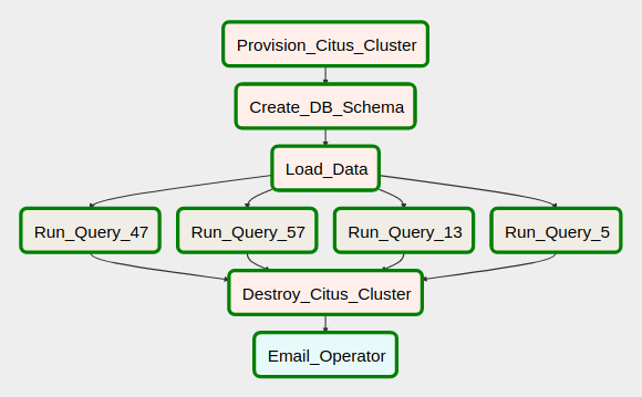
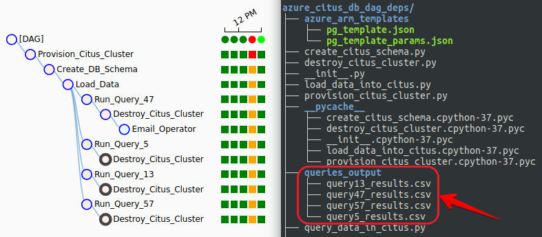
A similar type of workload is often used to create an idempotent pipeline which stitches together a number of tasks, including cloud infrastructure provisioning, data analytics, ETL/ELT activities etc. to design an end-to-end data management solution. The required DAG, with all its dependencies and activities should like as per the image below.

Sample Airflow Azure Cloud Pipeline Architecture

In order to provision the Azure resource groups and resources, I have created two JSON template files, also known as Azure Resource Manager (ARM) templates, which contain the required resources and their properties. ARM templates allow for declarative creation and deployment of any Azure infrastructure components e.g. virtual machines, hosted databases, storage accounts etc. along their properties and names. As the libraries used in the Python version of the Azure SDK directly mirror and consume Azure service’s REST endpoints, it’s quite easy to script out a repeatable deployment process using ARM templates as described in more details further along in this post. As part of the solution configuration, I have also created two SQL files which are used to create a suite of tables on the Citus cluster and run the queries, outputting the result sets into a local directory.

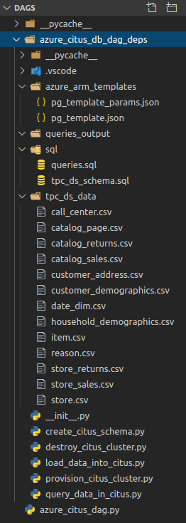The aforementioned files used to populate the Citus cluster schema are part of the TPC-DS benchmark data (scaling factor set to 1GB) and consist of a number of flat files in a CSV format. As we’re not going to recreate the whole TPC-DS benchmark suite of tests (this post is not intended to evaluate Citus database performance), to simplify the data loading process, I will only use a few of them (just over 800MB in size), which should provide us with enough data to run a few queries once the tables have been populated. To simplify this demonstration, all Python solution files as well as ARM JSON templates, SQL files and flat files data were moved into dags directory aka {AIRFLOW_HOME}/dags folder. Under typical scenario, data would not co-exists with configuration and solution files but for this exercise, I have nominated to structure the project as per the the directory breakdown on the left. Also, in a production environment, particularly one with many dag and task files, you would want to ensure that a consistent organizational structure is imposed across DAG folder and its sub-directories. As Airflow is such a versatile tool, depending on a specific use case, you may want to separate individual projects and their related hooks, operators, scripts and other files into their own respective folders etc.

With Airflow server up and running (installation and configuration instructions in the previous post HERE) and the files required to load into our Citus database schema staged in the solution directory we can start unpacking individual code samples used in the final DAG. As mentioned at the start, Citus database cluster, just as any other Azure resource, can be spun up declaratively using ARM template(s). You can peruse the content of the templates used in this demo as well as other artifacts in my publicly accessible OneDrive folder HERE.

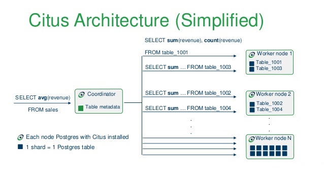
A quick word about Citus (now owned by Microsoft). Citus is an open source extension to PostgreSQL which distributes data and queries across multiple nodes. Because Citus is an extension to PostgreSQL (not a fork), it gives developers and enterprises a scale-out database while keeping the power and familiarity of a relational database. Citus horizontally scales PostgreSQL across multiple machines using sharding and replication. Its query engine parallelizes incoming SQL queries across these servers to enable super-fast responses on even very large datasets. I’m not very familiar with the service but there are many posts on the Internet describing some interesting projects Citus was used in, beating other competing technologies (TiDB, Apache Pinot, Apache Kylin, Apache Druid), partly due to its great SQL support and a large community of PostgreSQL users who are already familiar with the RDBMS it is based on e.g. HERE.

Now, let’s go through the individual scripts and unpack the whole solution piece by piece. The following Python script is using ARM templates to provision Azure resource group and a small Citus database cluster (single coordinator node and two worker nodes).

import adal
from timeit import default_timer as timer
from sys import platform
from msrestazure.azure_active_directory import AdalAuthentication
from msrestazure.azure_cloud import AZURE_PUBLIC_CLOUD
from azure.mgmt.resource.resources.models import (
    DeploymentMode,
    DeploymentProperties,
    Deployment,
)
from azure.mgmt.resource import ResourceManagementClient
from pathlib import Path, PurePosixPath
import json
import os

arm_template_location = PurePosixPath(
    "/home/airflow/airflow/dags/azure_citus_db_dag_deps/azure_arm_templates/pg_template.json"
)
arm_template_params_location = PurePosixPath(
    "/home/airflow/airflow/dags/azure_citus_db_dag_deps/azure_arm_templates/pg_template_params.json"
)

resource_group = "citus_svr_resource_group"
external_IP = os.popen("curl -s ifconfig.me").readline()
deployment_name = "azure_citus_deployment"

external_ip_params = {
    "name": "ClientIPAddress",
    "startIPAddress": external_IP,
    "endIPAddress": external_IP,
}
admin_login = {"value": "citus"}
admin_passwd = {"value": "your_citus_password"}

template = arm_template_location
params = arm_template_params_location

if template:
    with open(template, "r") as json_file_template:
        template = json.load(json_file_template)

if params:
    with open(params, "r") as json_file_template:
        params = json.load(json_file_template)
        params = {k: v for k, v in params["parameters"].items()}
        params["firewallRules"]["value"]["rules"][1] = external_ip_params
        params["administratorLogin"] = admin_login
        params["administratorLoginPassword"] = admin_passwd
        resource_group_location = params["location"]["value"]


# Tenant ID for your Azure Subscription
TENANT_ID = "123a27e2-7777-4d30-9ca2-ce960d430ef8"

# Your Service Principal App ID
CLIENT = "ae277f4e-882d-4f03-a0b5-b69275046123"

# Your Service Principal Password
KEY = "e7bbf0ed-d461-48c7-aace-c6a4822a123e"

# Your Azure Subscription ID
subscription_id = "1236a74c-dfd8-4b4d-b0b9-a355d2ec793e"

LOGIN_ENDPOINT = AZURE_PUBLIC_CLOUD.endpoints.active_directory
RESOURCE = AZURE_PUBLIC_CLOUD.endpoints.active_directory_resource_id

context = adal.AuthenticationContext(LOGIN_ENDPOINT + "/" + TENANT_ID)
credentials = AdalAuthentication(
    context.acquire_token_with_client_credentials, RESOURCE, CLIENT, KEY
)

client = ResourceManagementClient(credentials, subscription_id)


def create_citus_instance(resource_group):

    deployment_properties = {
        "mode": DeploymentMode.incremental,
        "template": template,
        "parameters": params,
    }

    deployment_async_operation = client.deployments.create_or_update(
        resource_group, deployment_name, deployment_properties
    )

    deployment_async_operation.wait()


def main():
    print("\nCreating Azure Resource Group...")
    start = timer()
    client.resource_groups.create_or_update(
        resource_group, {"location": resource_group_location}
    )
    print("Creating Citus Cluster...")
    create_citus_instance(resource_group)
    end = timer()
    time = round(end - start, 1)
    print("Total Elapsed Deployment Time = {t} seconds".format(
        t=format(time, ".2f")))


if __name__ == "__main__":
    main()

This file, called provision_citus_cluster.py, will be called from our Airflow DAG using PythonOperator and is the first step of our pipeline. The instance creation process should take a few minutes to provision and once created we can continue on and generate Citus cluster schema with all the required objects.

In order to populate Citus database with the flat files data we first need to create the desired schema (in this case called tpc_ds) and all the required objects. Even though this process will not be populating all tables (there are only thirteen flat files to be loaded), the script will create all TPC-DS benchmark objects using a simple SQL file containing all necessary DDL statements. The actual SQL file can be viewed and downloaded from my OneDrive folder so to keep this post concise, I will only include the Python script which parses the DDL SQL statements and executes those, creating all required tables. This operation (called from create_citus_schema.py file) will generate a second object in our DAG’s chain of tasks.

from pathlib import Path, PurePosixPath
from sys import platform
from psycopg2.extensions import ISOLATION_LEVEL_AUTOCOMMIT
import psycopg2
import sys

sql_schema = PurePosixPath(
    "/home/airflow/airflow/dags/azure_citus_db_dag_deps/sql/tpc_ds_schema.sql"
)

pg_args = {
    "user": "citus",
    "password": "your_citus_password",
    "host": "citussvrgroup-c.postgres.database.azure.com",
    "port": "5432",
    "database": "citus",
    "sslmode": "require",
}

pg_schema_name = "tpc_ds"


def get_sql(sql_schema):
    """
    Source operation types from the 'create_sqlite_schema' SQL file.
    Each operation is denoted by the use of four dash characters
    and a corresponding table DDL statement and store them in a dictionary
    (referenced in the main() function).
    """
    table_name = []
    query_sql = []

    with open(sql_schema, "r") as f:
        for i in f:
            if i.startswith("----"):
                i = i.replace("----", "")
                table_name.append(i.rstrip("\n"))

    temp_query_sql = []
    with open(sql_schema, "r") as f:
        for i in f:
            temp_query_sql.append(i)
        l = [i for i, s in enumerate(temp_query_sql) if "----" in s]
        l.append((len(temp_query_sql)))
        for first, second in zip(l, l[1:]):
            query_sql.append("".join(temp_query_sql[first:second]))
    sql = dict(zip(table_name, query_sql))
    return sql


def build_schema(sql_schema, pg_schema_name, **kwargs):
    connection = None
    try:
        connection = psycopg2.connect(**kwargs)
        cursor = connection.cursor()
        cursor.execute("SELECT version();")
        record = cursor.fetchone()
        if record:
            connection.set_isolation_level(ISOLATION_LEVEL_AUTOCOMMIT)
            cursor.execute(
                "CREATE SCHEMA IF NOT EXISTS {s};".format(
                    s=pg_schema_name)
            )
            conn_params = connection.get_dsn_parameters()
            if conn_params["dbname"] == "citus":
                sql = get_sql(sql_schema)
                ddls = sql.values()
                for s in ddls:
                    try:
                        cursor.execute(s)
                        connection.commit()
                    except (Exception, psycopg2.DatabaseError) as error:
                        print("Error while creating nominated database object", error)
                        sys.exit(1)
            else:
                raise Exception("Failed to connect to citus database.")

    except (Exception, psycopg2.Error) as error:
        print("Could not connect to your PostgreSQL instance.", error)
    finally:
        if connection:
            cursor.close()
            connection.close()


def main():
    build_schema(sql_schema, pg_schema_name, **pg_args)


if __name__ == "__main__":
    main()

Up next is our third task which loads text files data into the newly created database. The following Python code (solution file is called load_data_into_citus.py) is responsible for taking each of the staged flat files and copying those into the corresponding tables (in a sequential order).

import psycopg2
import os
import sys
from pathlib import Path, PurePosixPath
from psycopg2.extensions import ISOLATION_LEVEL_AUTOCOMMIT


tpc_ds_files = PurePosixPath(
    "/home/airflow/airflow/dags/azure_citus_db_dag_deps/tpc_ds_data/"
)

pg_schema_name = "tpc_ds"
encoding = "iso-8859-1"
pg_args = {
    "user": "citus",
    "password": "your_citus_password",
    "host": "citussvrgroup-c.postgres.database.azure.com",
    "port": "5432",
    "database": "citus",
    "sslmode": "require",
}


def load_data(tpc_ds_files, pg_schema_name, **kwargs):
    connection = None
    files = [f for f in os.listdir(tpc_ds_files) if f.endswith(".csv")]
    try:
        connection = psycopg2.connect(**kwargs)
        cursor = connection.cursor()
        cursor.execute("SELECT version();")
        record = cursor.fetchone()
        if record:
            connection.set_isolation_level(ISOLATION_LEVEL_AUTOCOMMIT)
            for file in files:
                schema_table_name = pg_schema_name + "." + file[:-4]
                with open(
                    os.path.join(tpc_ds_files, file), "r", encoding=encoding
                ) as f:
                    # next(f)  # Skip the header row
                    print(
                        "Truncating table {table_name}...".format(
                            table_name=schema_table_name
                        )
                    )
                    cursor.execute(
                        "TRUNCATE TABLE {table_name};".format(
                            table_name=schema_table_name
                        )
                    )
                    print(
                        "Copying file {file_name} into {table_name} table...\n".format(
                            file_name=file, table_name=schema_table_name
                        )
                    )
                    cursor.copy_from(f, schema_table_name, sep="|", null="")
                    file_row_rounts = sum(
                        1
                        for line in open(
                            os.path.join(tpc_ds_files, file),
                            encoding=encoding,
                            newline="",
                        )
                    )
                    cursor.execute(
                        "SELECT COUNT(1) FROM {tbl}".format(
                            tbl=schema_table_name)
                    )
                    record = cursor.fetchone()
                    db_row_counts = record[0]

                    if file_row_rounts != db_row_counts:
                        raise Exception(
                            "Table {tbl} failed to load correctly as record counts do not match: flat file: {ff_ct} vs database: {db_ct}.\
                            Please troubleshoot!".format(
                                tbl=schema_table_name,
                                ff_ct=file_row_rounts,
                                db_ct=db_row_counts,
                            )
                        )

    except Exception as e:
        print(e)
    finally:
        if connection:
            cursor.close()
            connection.close()


def main():
    load_data(tpc_ds_files, pg_schema_name, **pg_args)


if __name__ == "__main__":
    main()

As you may expect, each one of the aforementioned operations needs to be executed sequentially as there are clear dependencies across each of the steps outlined above i.e. database objects cannot be populated without the schema being created in the first place and likewise, database schema cannot be created without the database instance being present. However, when it comes to SQL queries execution, Citus was designed to crunch large volumes of data concurrently. Our next set of operation will calculate and generate four separate SQL results and stage those as CSV files inside the ‘queries_output’ folder. Please also note that this post does not look into Citus cluster performance and is not concerned with the queries execution times. We are not attempting to tune the way the data is distributed across the nodes or adjust any configuration parameters as the main purpose of this post is to highlight Airflow functionality and design patterns for the above scenarios.

import psycopg2
import os
import sys
import csv
from pathlib import Path, PurePosixPath


sql_queries_file = PurePosixPath("/home/airflow/airflow/dags/azure_citus_db_dag_deps/sql/queries.sql")
sql_output_files_dir = PurePosixPath(
        "/home/airflow/airflow/dags/azure_citus_db_dag_deps/queries_output/"
    )

pg_schema_name = "tpc_ds"
encoding = "iso-8859-1"
pg_args = {
    "user": "citus",
    "password": "your_citus_password",
    "host": "citussvrgroup-c.postgres.database.azure.com",
    "port": "5432",
    "database": "citus",
    "sslmode": "require",
}


def get_sql(sql_queries_file):
    query_number = []
    query_sql = []

    with open(sql_queries_file, "r") as f:
        for i in f:
            if i.startswith("----"):
                i = i.replace("----", "")
                query_number.append(i.rstrip("\n"))
    temp_query_sql = []
    with open(sql_queries_file, "r") as f:
        for i in f:
            temp_query_sql.append(i)
        l = [i for i, s in enumerate(temp_query_sql) if "----" in s]
        l.append((len(temp_query_sql)))
        for first, second in zip(l, l[1:]):
            query_sql.append("".join(temp_query_sql[first:second]))
    sql = dict(zip(query_number, query_sql))
    return sql


def main():
    query_sql = sql.get(param).rstrip()
    query_sql = query_sql[:-1] # remove last semicolon
    output_file_name = param.lower() + "_results.csv"
    try:
        connection = psycopg2.connect(**pg_args)
        cursor = connection.cursor()
        cursor.execute("SELECT version();")
        record = cursor.fetchone()
        if record:
            sql_for_file_output = "COPY ({0}) TO STDOUT WITH CSV DELIMITER '|';".format(query_sql)
            with open(os.path.join(sql_output_files_dir, output_file_name), "w") as output_file:
                cursor.copy_expert(sql_for_file_output, output_file)
    except Exception as e:
        print(e)
    finally:
        if connection:
            cursor.close()
            connection.close()


if __name__ == "__main__":
    if len(sys.argv[1:]) == 1:
        sql = get_sql(sql_queries_file)
        param = sys.argv[1]
        query_numbers = [q for q in sql]
        if param not in query_numbers:
            raise ValueError(
                "Incorrect argument given. Choose from the following numbers: {q}".format(
                    q=" or ".join(query_numbers)
                )
            )
        else:
            param = sys.argv[1]
            main()
    else:
        raise ValueError(
            "Too many arguments given. Looking for <query number> numerical value."
        )

The above code is executed using BashOperator rather than PythonOperator, as each query is run with a parameter passed to the executing script, indicating the SQL query number. Additionally, each query output (the result set) is staged as a CSV file on the local drive so that at the end of the pipeline execution we should end up with four flat files in the queries_output folder.

Last but not least, we will initialize the ‘clean-up’ step, where Citus cluster resource group and all its corresponding services will be terminated to avoid incurring additional cost and send an email to a nominated email address, notifying administrator of the successful pipeline execution completion. The following Python code terminates and deletes all resources created in this process.

import adal
from timeit import default_timer as timer
from sys import platform
from msrestazure.azure_active_directory import AdalAuthentication
from msrestazure.azure_cloud import AZURE_PUBLIC_CLOUD
from azure.mgmt.resource.resources.models import (
    DeploymentMode,
    DeploymentProperties,
    Deployment,
)
from azure.mgmt.resource import ResourceManagementClient

resource_group = "citus_svr_resource_group"


# Tenant ID for your Azure Subscription
TENANT_ID = "123a27e2-7777-4d30-9ca2-ce960d430ef8"

# Your Service Principal App ID
CLIENT = "ae277f4e-882d-4f03-a0b5-b69275046123"

# Your Service Principal Password
KEY = "e7bbf0ed-d461-48c7-aace-c6a4822a123e"

# Your Azure Subscription ID
subscription_id = "1236a74c-dfd8-4b4d-b0b9-a355d2ec793e"

LOGIN_ENDPOINT = AZURE_PUBLIC_CLOUD.endpoints.active_directory
RESOURCE = AZURE_PUBLIC_CLOUD.endpoints.active_directory_resource_id

context = adal.AuthenticationContext(LOGIN_ENDPOINT + "/" + TENANT_ID)
credentials = AdalAuthentication(
    context.acquire_token_with_client_credentials, RESOURCE, CLIENT, KEY
)

client = ResourceManagementClient(credentials, subscription_id)


def main():
    client.resource_groups.delete(resource_group)


if __name__ == "__main__":
    main()

There are many ways one can script out email notification dispatch using Python, however, Airflow provides out-of-the-box functionality in the form of EmailOperator. For this demonstration I decided to use my personal Gmail address which required a slight change to the airflow.cfg (Airflow configuration) file as well as creating a Google account App Password. More on the process of creating App Password can be found HERE. The following changes to the Airflow configuration file are required (in addition to DAG-specyfic email task definition) to enable EmailOperator functionality with Gmail-specyfic email address.

smtp_host = smtp.gmail.com
smtp_user = your_gmail_email_address@gmail.com
smtp_password = your_app_password
smtp_port = 587
smtp_mail_from = Airflow

The final piece of the puzzle is the actual DAG file responsible for individual tasks definition as per my previous introductory post to Airflow HERE. The following Python code is responsible for defining DAG arguments, individual tasks and the order they should be executed in. Notice that some Python tasks are executed using BashOperator instead of PythonOperator. That’s because those scripts are run with an argument passed to them using Python sys module argv list, denoting query number which the script is to run. Also, those tasks need to include full path to where the script is located. In contrast, PythonOperator only requires a Python callable to be included.

from airflow import DAG
from airflow.operators.bash_operator import BashOperator
from airflow.operators.python_operator import PythonOperator
from datetime import datetime, timedelta
from airflow.operators.email_operator import EmailOperator
from azure_citus_db_dag_deps import create_citus_schema
from azure_citus_db_dag_deps import load_data_into_citus
from azure_citus_db_dag_deps import provision_citus_cluster
from azure_citus_db_dag_deps import destroy_citus_cluster


default_args = {
    'owner': 'Airflow',
    'depends_on_past': False,
    'start_date': datetime(2019, 6, 1),
    'email': ['airflow@example.com'],
    'email_on_failure': False,
    'email_on_retry': False,
    'retries': 0,
    # 'retry_delay': timedelta(minutes=5),
    # 'queue': 'bash_queue',
    # 'pool': 'backfill',
    # 'priority_weight': 10,
    # 'end_date': datetime(2016, 1, 1),
}

with DAG('Azure_Citus_Database_Job', default_args=default_args, schedule_interval=None) as dag:
    provisioning_citus_cluster = PythonOperator(
        task_id="Provision_Citus_Cluster",
        python_callable=provision_citus_cluster.main)
    creating_citus_schema = PythonOperator(
        task_id="Create_DB_Schema", python_callable=create_citus_schema.main)
    loading_csv_data = PythonOperator(
        task_id="Load_Data", python_callable=load_data_into_citus.main)
    executing_sql_query_5 = BashOperator(
        task_id="Run_Query_5", bash_command='python ~/airflow/dags/azure_citus_db_dag_deps/query_data_in_citus.py Query5'
    )
    executing_sql_query_13 = BashOperator(
        task_id="Run_Query_13", bash_command='python ~/airflow/dags/azure_citus_db_dag_deps/query_data_in_citus.py Query13'
    )
    executing_sql_query_47 = BashOperator(
        task_id="Run_Query_47", bash_command='python ~/airflow/dags/azure_citus_db_dag_deps/query_data_in_citus.py Query47'
    )
    executing_sql_query_57 = BashOperator(
        task_id="Run_Query_57", bash_command='python ~/airflow/dags/azure_citus_db_dag_deps/query_data_in_citus.py Query57'
    )
    destroying_citus_cluster = PythonOperator(
        task_id="Destroy_Citus_Cluster", python_callable=destroy_citus_cluster.main)

    emailing_operator = EmailOperator(
        task_id="Email_Operator",
        to="your_gmail_email_address@gmail.com",
        subject="Airflow Message",
        html_content="""<h1>Congratulations! All your tasks are now completed.</h1>"""
    )

provisioning_citus_cluster >> creating_citus_schema >> loading_csv_data >> executing_sql_query_5 >> destroying_citus_cluster >> emailing_operator
provisioning_citus_cluster >> creating_citus_schema >> loading_csv_data >> executing_sql_query_13 >> destroying_citus_cluster >> emailing_operator
provisioning_citus_cluster >> creating_citus_schema >> loading_csv_data >> executing_sql_query_47 >> destroying_citus_cluster >> emailing_operator
provisioning_citus_cluster >> creating_citus_schema >> loading_csv_data >> executing_sql_query_57 >> destroying_citus_cluster >> emailing_operator

Now that we have everything in place we can kick this DAG off and wait for the pipeline to go through its individual execution steps, concluding with the queries output files staged in the nominated folder as well as the email sent to the Gmail address we specified.

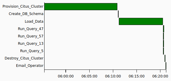
When finished, Airflow can provide us with the Gantt chart breakdown on how long individual tasks took which helps with pinpointing slow-running processes and gives us a good overview of time consumed across each step.

Additionally, we can now see the DAG tree view completion status (green = success, red = failure) for each run and each step, the four output files staged in the nominated directory with expected queries result sets persisted and finally, the email notification sent out on pipeline successful completion.

Conclusion

This concludes this short series outlining some of the core functionality of Airflow workflow management system. From the short time I spent with Airflow it seems like it fills the void for a robust, open-source, configuration-as-code platform which can be used across many different application, not just ETL/ELT e.g. automating DevOps operations, machine learning pipelines, scheduler replacement etc. Its documentation is passable, it has a fairly mild learning curve, it’s fairly extensible and scalable, has a good management interface and its adoption rate, particularly in the startup community, is high as it is slowly becoming the de facto platform for programmatic workloads authoring/scheduling. Data engineering field has been changing rapidly over the last decade, competition is rife and I’m not sure whether Airflow will be able to sustain its momentum in years to come. However, given its current rise to stardom, easily superseding tools such as Apache Oozie or Luigi, anyone in the field of Data Engineering should be at least familiar with it.

Posted in: Cloud Computing, MPP RDBMS, Programming, SQL

Tags: Azure, Cloud Computing, Data Warehouse, ETL, MPP RDBMS, Programming, Python, SQL

Kicking the Tires on Airflow, Apache’s workflow management platform – Architecture Overview, Installation and sample Azure Cloud Deployment Pipeline in Python (Part 1)

April 13th, 2020 / No Comments » / by admin

Note: Part 2 can be found HERE and all files used in this tutorial can be downloaded from HERE.

Ever since I can remember, most of ETL or ELT jobs I was tasked with architecting and/or developing were based on batch processing. Nowadays, the trend is leaning heavily towards streaming or semi-real time processing where possible, but the complex nature of those systems and the relative immaturity of the ecosystems they promote still means that most business are reluctant to transition away from an old-school batch processing. The last few years have seen more of a Lambda deployment (hybrid of real-time and batch workloads) but most business requirements for data availability in SMB scenarios hardly go beyond ‘next day is fine’ approach. This, however, does not mean that the platforms themselves have not evolved and that the tooling around how these pipelines are structured have not moved on with time. Most GUI based applications e.g. SSIS, Pentaho, Talend etc. are evolving and morphing into cloud-first solutions and major vendors are launching new features to keep up with the insatiable need for speed of major cloud behemoths. Also, the design patterns and ways which ETL/ELT is architected is undergoing a major transformation, with code and configuration-based deployment taking over drag-and-drop and point-and-click applications. Graphical interface-based tools are arguably easier to debug but with a plethora of new data sources to integrate with, tools like Amazon’s Glue or Apache Airflow are slowly emerging as favourites with the new breed of data engineers and analytics-driven companies alike.

In spite of Airflow being only few years old (project was open-sourced in 2015), it has become Apache’s Top Level Project a year later, with over 1K contributors, 15K stars on Github and close to 10K commits. Airflow has been used successfully in production by both: countless number of smaller startups and big corporations alike (AirBnB, Slack, Square, Robinhood) and its popularity even kickstrated Google to create a managed version called Cloud Composer, running on GCP. Airflow’s versatility and flexibility also allows it to be used for workloads not associated with building ETL/ELT data pipelines e.g. automating DevOps operations, machine learning pipelines, scheduler replacement etc.

Some of the main reasons why Airflow has been gaining momentum across data engineering communities and is slowly superseding tools such as Apache Oozie or Luigi include the following:

• Airflow is dynamic – DAGs in Airflow are dynamic and flexible in nature. As Airflow pipelines are configured as code (Python), many knobs and switches are available to its developers and nearly any aspect of the pipeline development can be customised and tuned. Also, DAGs provide a nice abstraction to a series of operations
• Airflow is extensible – Airflow provides large number of operators and executors thus allowing any tasks (not just ETL) to be scheduled and executed. In case a specific operator/executor is not available out of the box, Airflow extensible architecture allows defining your own with relative ease
• Airflow is scalable – Airflow modular architecture, built-in provisions for configuring a choice of different message queueing systems and executors e.g. RabbitMQ, Celery, Dask, Mesos, multi-node cluster configuration and Kubernetes-based tasks execution model allow for tasks to be deployed and run across number of machines/VMs/containers. While Airflow is not designed to perform any computation itself and tasks can be executed in a sequential manner, Airflow is designed to spread the workloads and maximise computation resources availability
• Airflow has a good monitoring and management interface – Airflow provides a monitoring and managing interface, where it is possible to have a quick overview of the status of the different tasks, as well as have the possibility to trigger and clear tasks or DAGs runs
• Airflow is open source – due to the fact that Airflow is not a commercial product and Airflow’s community is very active, the tool receives a steady stream of updates and code contributions, further extending its functionality

Airflow Architecture

Apache Airflow is an open-source workflow management platform. It started at Airbnb in October 2014 as a solution to manage the company’s increasing complex workflows. Creating Airflow allowed Airbnb to programmatically author and schedule their workflows and monitor them via the built-in Airflow user interface. From the beginning, the project was made open source, becoming an Apache Incubator project in March 2016 and a Top-Level Apache Software Foundation project in January 2019.

Building on the popularity of Python as the de facto programming language for data, Airflow is written in Python and workflows are created via Python scripts. Airflow is designed under the principle of “configuration as code” where the Airflow scheduler periodically checks whether or not criteria for running tasks have been met, have other conditions for execution been met etc. according to the dependencies defined in directed acyclic graphs (DAGs). Once all criteria have been met, this fact is recorded in the database and Airflow worker pick up and run jobs with their loads properly balanced. Depending on the choice of setup this worker process can be a single process on a single machine, multiple processes on a single machine or multiple processes distributed across multiple machines. All job information is stored in the meta DB, which is updated in a timely manner. The users can monitor their jobs via a shiny Airflow web UI and/or the logs. A sample Airflow architecture with all its key components and services is as per the image below.

In Airflow, a DAG – or a Directed Acyclic Graph – is a collection of all the tasks you want to run, organized in a way that reflects their relationships and dependencies. For example, a simple DAG could consist of three tasks: A, B, and C. It could say that A has to run successfully before B can run, but C can run anytime. It could say that task A times out after 5 minutes, and B can be restarted up to 5 times in case it fails. It might also say that the workflow will run every night at 10pm, but shouldn’t start until a certain date. In this way, a DAG describes how you want to carry out your workflow; but notice that we haven’t said anything about what we actually want to do! A, B, and C could be anything. Maybe A prepares data for B to analyze while C sends an email. Or perhaps A monitors your location so B can open your garage door while C turns on your house lights. The important thing is that the DAG isn’t concerned with what its constituent tasks do; its job is to make sure that whatever they do happens at the right time, or in the right order, or with the right handling of any unexpected issues. DAGs are defined in standard Python files that are placed in Airflow’s ‘dags’ folder. Airflow will execute the code in each file to dynamically build the DAG objects. You can have as many DAGs as you want, each describing an arbitrary number of tasks. In general, each one should correspond to a single logical workflow.

Installing Airflow

There are a lot of really detailed and comprehensive posts on the internet describing step-by-step process for Airflow installation across various platforms so in this post I will refrain from looking into all the different ways Airflow can be deployed. For the purpose of this demo, I will spin up Ubuntu micro VM on the Henzner VPS, install Anaconda Python distribution and PostgreSQL database (used for Airflow metadata). The process is fairly straightforward, and all these tasks can be accomplished using your favorite terminal with just a few commands.

#create 'airflow' user
sudo adduser airflow
sudo usermod -aG sudo airflow
su - airflow

#download and install Anaconda and PostgreSQL
curl -O https://repo.anaconda.com/archive/Anaconda3-2019.10-Linux-x86_64.sh
bash Anaconda3-2019.10-Linux-x86_64.sh
conda install -c conda-forge azure-cli-core
sudo apt-get update --fix-missing
sudo apt-get install build-essential autoconf
sudo apt-get install postgresql postgresql-contrib
sudo service postgresql start

#set up database user, database and its permissions
sudo -u postgres psql
CREATE USER airflow PASSWORD 'YourTopSecretPassword';
CREATE DATABASE airflow;
GRANT ALL PRIVILEGES ON ALL TABLES IN SCHEMA public TO airflow;

#change PostgreSQL config to accept Airflow connections
sudo nano /etc/postgresql/10/main/pg_hba.conf

#change 'IPv4 local connections' value to the following:
host all all 0.0.0.0/0 trust
sudo nano /etc/postgresql/10/main/postgresql.conf

#change listen_addresses = 'localhost' to the following value:
listen_addresses = '*'

#restart PostgreSQL service
sudo service postgresql restart

#install Airflow and its packages
export AIRFLOW_HOME=~/airflow
pip install "apache-airflow[postgres]"
airflow initdb

#update airflow config values
cd airflow
sudo nano airflow.cfg

#change default value for the executor (SequentialExecutor) to the following value:
executor = LocalExecutor

#change default value for sql_alchemy_conn to the following value:
sql_alchemy_conn = postgresql+psycopg2://airflow@localhost:5432/airflow

#ensure that the following connection pooling parameter is set to True:
sql_alchemy_pool_enabled = True

#change from default Sqlite database to PostgreSQL
airflow initdb

#start Airflow services
airflow webserver
airflow scheduler

Once completed and web server is up and running, we should be able to access Airflow admin panel accessing the following URL: your_server_up_address:8080/admin. This process runs a simple Flask application which reads the state of all tasks from the metadata database and renders these states for the Web UI. Also, given that the default Sqlite metadata database has been replaced with a more robust PostgreSQL instance, the following airflow schema was generated (click on image to enlarge).

To demonstrate the internal working of Airflow and some of its key architectural principles it’s probably best to create a simple, multi-task workflow. In this two-part post I will be creating two separate DAGs – one to provide a brief overview of the DAG file template in its simplest form and another one which will include a more comprehensive workflow interacting with a public cloud resources as well as local data.

Airflow Sample Workflow – Basic DAG

Let’s start with the most basic workflow and introduce the anatomy of the pipeline creation, DAG definition file and individual tasks. One thing to remember is that this Airflow Python script is just a configuration file specifying the DAG’s structure as code. The actual tasks defined here will run in a different context from the context of this script. Different tasks run on different workers at different points in time, which means that this script cannot be used to cross communicate between tasks (with the exception of Xcom – a more advanced Airflow concept). An Airflow pipeline is just a Python script that happens to define an Airflow DAG object. Let’s start by importing the libraries we will need.

# The DAG object; we'll need this to instantiate a DAG
from airflow import DAG

# Operators; we need this to operate!
from airflow.operators.bash_operator import BashOperator

When creating a DAG and some tasks, we have the choice to explicitly pass a set of arguments to each task’s constructor (which would become redundant), or (better!) we can define a dictionary of default parameters that we can use when creating tasks.

from datetime import datetime, timedelta

default_args = {
    'owner': 'Airflow',
    'depends_on_past': False,
    'start_date': datetime(2020, 1, 30),
    'email': ['airflow@example.com'],
    'email_on_failure': False,
    'email_on_retry': False,
    'retries': 1,
    'retry_delay': timedelta(minutes=5),
    # 'queue': 'bash_queue',
    # 'pool': 'backfill',
    # 'priority_weight': 10,
    # 'end_date': datetime(2020, 1, 30),
}

We’ll need a DAG object to nest our tasks into. Here we pass a string that defines the dag_id, which serves as a unique identifier for your DAG. We also pass the default argument dictionary that we just defined and define a schedule_interval of 1 day for the DAG.

dag = DAG(
    'tutorial', default_args=default_args, schedule_interval=timedelta(days=1))

Tasks are generated when instantiating operator objects. An object instantiated from an operator is called a constructor. The first argument task_id acts as a unique identifier for the task.

t1 = BashOperator(
    task_id='print_date',
    bash_command='date',
    dag=dag)

t2 = BashOperator(
    task_id='sleep',
    bash_command='sleep 5',
    retries=3,
    dag=dag)

Notice how we pass a mix of operator specific arguments (bash_command) and an argument common to all operators (retries) inherited from BaseOperator to the operator’s constructor. This is simpler than passing every argument for every constructor call. Also, notice that in the second task we override the retries parameter with 3.

Airflow leverages the power of Jinja Templating and provides the pipeline author with a set of built-in parameters and macros. Airflow also provides hooks for the pipeline author to define their own parameters, macros and templates. This tutorial barely scratches the surface of what you can do with templating in Airflow, but the goal of this section is to let you know this feature exists, get you familiar with double curly brackets, and point to the most common template variable: {{ ds }} (today’s “date stamp”).

templated_command = """
    {% for i in range(5) %}
        echo "{{ ds }}"
        echo "{{ macros.ds_add(ds, 7) }}"
        echo "{{ params.my_param }}"
    {% endfor %}
"""

t3 = BashOperator(
    task_id='templated',
    bash_command=templated_command,
    params={'my_param': 'Parameter I passed in'},
    dag=dag)

Notice that the templated_command contains code logic in {% %} blocks, references parameters like {{ ds }}, calls a function as in {{ macros.ds_add(ds, 7)}}, and references a user-defined parameter in {{ params.my_param }}. The params hook in BaseOperator allows you to pass a dictionary of parameters and/or objects to your templates. Files can also be passed to the bash_command argument, like bash_command=’templated_command.sh’, where the file location is relative to the directory containing the pipeline file. This may be desirable for many reasons, like separating your script’s logic and pipeline code, allowing for proper code highlighting in files composed in different languages, and general flexibility in structuring pipelines. It is also possible to define your template_searchpath as pointing to any folder locations in the DAG constructor call. Using that same DAG constructor call, it is possible to define user_defined_macros which allow you to specify your own variables. For example, passing dict(foo=’bar’) to this argument allows you to use {{ foo }} in your templates. Moreover, specifying user_defined_filters allow you to register you own filters. For example, passing dict(hello=lambda name: ‘Hello %s’ % name) to this argument allows you to use {{ ‘world’ | hello }} in your templates.

Now that we have tasks t1, t2 and t3 that do not depend on each other we need to define a chain of dependencies between them. The following example shows few different ways this can be achieved by.

t1.set_downstream(t2)

# This means that t2 will depend on t1
# running successfully to run.
# It is equivalent to:
t2.set_upstream(t1)

# The bit shift operator can also be
# used to chain operations:
t1 >> t2

# And the upstream dependency with the
# bit shift operator:
t2 << t1 # Chaining multiple dependencies becomes # concise with the bit shift operator: t1 >> t2 >> t3

# A list of tasks can also be set as
# dependencies. These operations
# all have the same effect:
t1.set_downstream([t2, t3])
t1 >> [t2, t3]
[t2, t3] << t1

Note that when executing your script, Airflow will raise exceptions when it finds cycles in your DAG or when a dependency is referenced more than once. At this point our code should look something like this.

from airflow import DAG
from airflow.operators.bash_operator import BashOperator
from datetime import datetime, timedelta


default_args = {
    'owner': 'Airflow',
    'depends_on_past': False,
    'start_date': datetime(2015, 6, 1),
    'email': ['airflow@example.com'],
    'email_on_failure': False,
    'email_on_retry': False,
    'retries': 1,
    'retry_delay': timedelta(minutes=5),
    # 'queue': 'bash_queue',
    # 'pool': 'backfill',
    # 'priority_weight': 10,
    # 'end_date': datetime(2016, 1, 1),
}

dag = DAG(
    'tutorial', default_args=default_args, schedule_interval=timedelta(days=1))

# t1, t2 and t3 are examples of tasks created by instantiating operators
t1 = BashOperator(
    task_id='print_date',
    bash_command='date',
    dag=dag)

t2 = BashOperator(
    task_id='sleep',
    bash_command='sleep 5',
    retries=3,
    dag=dag)

templated_command = """
    {% for i in range(5) %}
        echo "{{ ds }}"
        echo "{{ macros.ds_add(ds, 7)}}"
        echo "{{ params.my_param }}"
    {% endfor %}
"""

t3 = BashOperator(
    task_id='templated',
    bash_command=templated_command,
    params={'my_param': 'Parameter I passed in'},
    dag=dag)

t2.set_upstream(t1)
t3.set_upstream(t1)

Finally, when our DAG file is saved into the default folder location, Airflow scheduler should pick it up and display its graph view (showing all its dependencies) as per the image below.

This concludes a brief Airflow architecture overview and a sample pipeline built tutorial. For information on more complex DAGs e.g. involving dynamic provisioning of Azure cloud services (Citus database cluster) please refer to the second part of this post HERE.

Posted in: Azure, Cloud Computing, MPP RDBMS, Programming, SQL

Tags: Airflow, Azure, Cloud Computing, ETL, Programming, Python