Data Analysis with Dask – A Python Scale-Out, Parallel Computation Framework For Big Data
July 14th, 2019 / No Comments » / by admin
Introduction
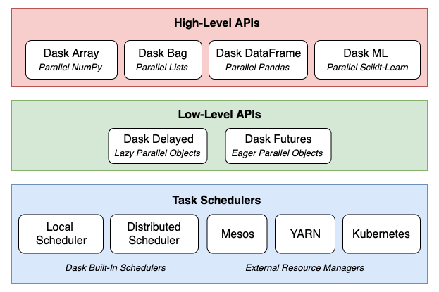
The jury is still out on whether Python emerged as the clear favourite language for all things data but from my personal experience I am witnessing more and more folks working in the field of data wrangling gravitating towards Python rich libraries ecosystem, particularly the so-called Python Open Data Science Stack i.e. Pandas, NumPy, SciPy, and Scikit-learn and away from the industry stalwarts e.g. Fortran, Matlab and Octave. Alongside new tooling and frameworks development, computers have continued to become ever more powerful. This makes it easy to produce, collect, store, and process far more data than before, all at a price that continues to march downward. But, this deluge of data now has many organisations questioning the value of collecting and storing all that data. Working with the Python Open Data Science Stack, data scientists often turn to tools like Pandas for data cleaning and exploratory data analysis, SciPy and NumPy to run statistical tests on the data, and Scikit-Learn to build predictive models. This all works well for relatively small-sized datasets that can comfortably fit into RAM. But, because of the shrinking expense of data collection and storage, data scientists are more frequently working on problems that involve analysing enormous datasets. These tools have upper limits to their feasibility when working with datasets beyond a certain size. Once the threshold is crossed, it is difficult to extract meaning out of data due to painfully long run times – even for the simplest of calculations, unstable code, and unwieldy workflows. Large datasets are datasets that can neither fit in RAM nor can fit in a single computer’s persistent storage. These datasets are typically above 1 terabyte in size, and depending on the problem, can reach into petabytes and beyond. Pandas, NumPy, and Scikit-Learn are not suitable at all for datasets of this size, as they were not inherently built to operate on distributed datasets. Enter Dask. Launched in late 2014 by Matthew Rocklin with aims to bring native scalability to the Python Open Data Science Stack and overcome its single machine restrictions Dask has proven to be a great alternative to Big Data frameworks, which sometimes require specialised expertise and maintenance/configuration overhead e.g. Apache Spark. Dask consists of several different components and APIs, which can be categorised into three layers: task schedulers, low-level APIs, and high-level APIs.
What makes Dask so powerful is how these components and layers are built on top of one another. At the core are the task schedulers, which coordinate and monitor execution of computations across CPU cores and machines. These computations are represented in code either as Dask Delayed objects or Dask Futures objects (the key difference is the former are evaluated lazily – meaning they are evaluated just-in-time when the values are needed, while the latter are evaluated eagerly – meaning they are evaluated in real-time regardless of if the value is needed immediately or not). Dask’s high-level APIs offer a layer of abstraction over Delayed and Futures objects. Operations on these high-level objects result in many parallel low-level operations managed by the task schedulers, which provides a seamless experience for the user.
As a result, Dask can scale out data processing computation across multiple machines and hundreds of terabytes of data efficiently. Dask can also enable efficient parallel computations on single machines by leveraging their multi-core CPUs and streaming data efficiently from disk. It can run on a distributed cluster, but it doesn’t have to. Dask allows you to swap out the cluster for single-machine schedulers which are surprisingly lightweight, require no setup, and can run entirely within the same process as the user’s session. To avoid excess memory use, Dask is good at finding ways to evaluate computations in a low-memory footprint when possible by pulling in chunks of data from disk, doing the necessary processing, and throwing away intermediate values as quickly as possible. This lets analysts perform computations on moderately large datasets (100GB+) even on relatively low-power laptops. This requires no configuration and no setup, meaning that adding Dask to a single-machine computation adds very little cognitive overhead.
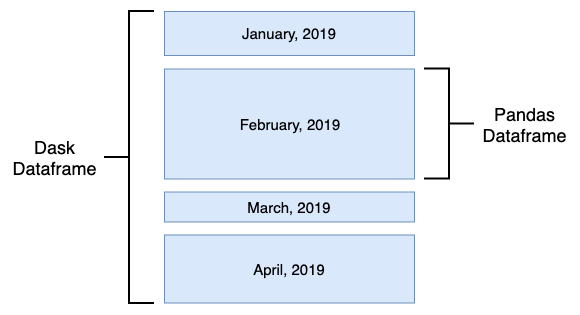
Even though Dask set of APIs can be utilised to tackle problems across a wide range of spectrum e.g. multi-dimensional data analysis, scalable machine learning training and prediction on large models etc., one of its primary uses is to enable Pandas-like workflows i.e. enabling applications in time series, business intelligence and general data crunching on big data. Like Pandas, Dask also utilises a concept of a DataFrame, with most functionality overlapping that of Pandas. A Dask DataFrame is a large parallel DataFrame composed of many smaller Pandas DataFrames, split along the index. These Pandas DataFrames may live on disk for larger-than-memory computing on a single machine, or on many different machines in a cluster. One Dask DataFrame operation triggers many operations on the constituent Pandas DataFrames.
Testing Methodology and Results
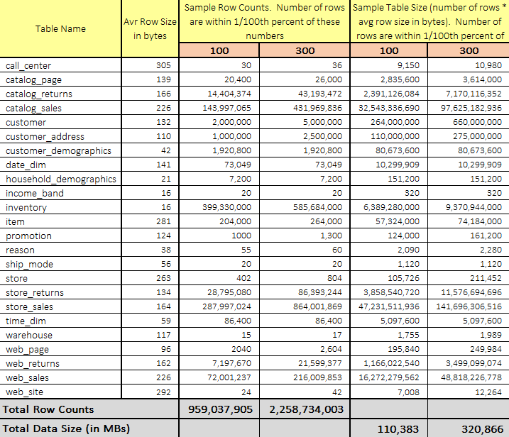
Let’s look whether we can benefit from using Dask and its parallel computation functionality to process data generated by the TPC-DS benchmark faster. There are a few other data sets and methodologies that can be used to gauge data storage and processing system’s performance e.g. TLC Trip Record Data released by the New York City Taxi, however, TPC-approved benchmarks have long been considered as the most objective, vendor-agnostic way to perform data-specific hardware and software comparisons, capturing the complexity of modern business processing to a much greater extent than its predecessors.
Firstly, let’s load the 10GB TPC-DS flat files into a Sqlite database using Python script. The following code takes two arguments – 1st one for how the data should be loaded i.e. using Python pandas module or csv module and 2nd one as a comma separated list of file names to be loaded (alternatively ‘all’ value can be passed if all files are to be loaded). This script also builds the database schema which definition is stored in a separate SQL file, creates indexes on some of the tables to speed up subsequent data extraction and finally, creates 10 views – each containing an increment of 1 million records for testing purposes. When loaded all files sequentially, it took around 1 hour to process and generate Sqlite database, which ends up being around 17GB is size.
#!/usr/bin/python
import sqlite3
import sys
import os
import csv
import time
import pandas as pd
import argparse

tpc_ds_files = '/Volumes/SSHD2/10GB'
tpc_ds_files_processed = '/Volumes/SSHD2/10GB/Processed'
dbsqlite_location = '/Volumes/SSHD2/10GB/DB'
dbsqlite_filename = 'testdb.db'
schema_sql_location = '/Volumes/SSHD2/10GB/DB'
schema_sql_filename = 'create_sqlite_schema.sql'
view_sql_location = '/Volumes/SSHD2/10GB/DB'

view_sql_filename = 'create_view.sql'
encoding = 'iso-8859-1'
view_sql_name = 'vw_test_data'
encoding = 'iso-8859-1'
indexes = [['store_sales', 'ss_sold_date_sk'],
           ['store_sales', 'ss_addr_sk'],
           ['store_sales', 'ss_item_sk'],
           ['store_sales', 'ss_store_sk'],
           ['date_dim', 'd_day_name']]
record_counts = ['1000000',
                 '2000000',
                 '3000000',
                 '4000000',
                 '5000000',
                 '6000000',
                 '7000000',
                 '8000000',
                 '9000000',
                 '10000000']
methods = ['use_pandas', 'use_csv']
view_sql_filename = 'create_view.sql'
view_sql_name = 'vw_test_data'
encoding = 'iso-8859-1'


def get_sql(sql_statements_file_path):
    """
    Source operation types from the 'create_sqlite_schema' SQL file.
    Each operation is denoted by the use of four dash characters
    and a corresponding table DDL statement and store them in a dictionary
    (referenced in the main() function).
    """
    table_name = []
    query_sql = []

    with open(sql_statements_file_path, "r") as f:
        for i in f:
            if i.startswith("----"):
                i = i.replace("----", "")
                table_name.append(i.rstrip("\n"))

    temp_query_sql = []
    with open(sql_statements_file_path, "r") as f:
        for i in f:
            temp_query_sql.append(i)
        l = [i for i, s in enumerate(temp_query_sql) if "----" in s]
        l.append((len(temp_query_sql)))
        for first, second in zip(l, l[1:]):
            query_sql.append("".join(temp_query_sql[first:second]))
    sql = dict(zip(table_name, query_sql))
    return sql


def RemoveTrailingChar(row_limit, file, encoding, tpc_ds_files, tpc_ds_files_processed):
    """
    Remove trailing '|' characters from the files generated by the TPC-DS utility
    as they intefere with Sqlite load function.
    """
    line_numer = row_limit
    lines = []
    with open(os.path.join(tpc_ds_files, file), 'r', encoding=encoding) as r,\
            open(os.path.join(tpc_ds_files_processed, file), 'w', encoding=encoding) as w:
        for line in r:
            line.encode(encoding).strip()
            if line.endswith('|\n'):
                lines.append(line[:-2]+"\n")
                if len(lines) == line_numer:
                    w.writelines(lines)
                    lines = []
        w.writelines(lines)


def SourceFilesRename(tpc_ds_files_processed):
    """"
    Rename files extensions from .dat to .csv
    """
    for file in os.listdir(tpc_ds_files_processed):
        if file.endswith(".dat"):
            os.rename(os.path.join(tpc_ds_files_processed, file),
                      os.path.join(tpc_ds_files_processed, file[:-4]+'.csv'))


def BuildSchema(conn, arg_method, arg_tables, dbsqlite_location, dbsqlite_filename, sql):
    """
    Build Sqlite database schema based on table names passed
    """
    if arg_tables[0] == 'all':
        sql = sql.values()
    else:
        sql = {x: sql[x] for x in sql if x in arg_tables}
        sql = sql.values()
    for s in sql:
        try:
            conn.executescript(s)
        except sqlite3.OperationalError as e:
            print(e)
            conn.rollback()
            sys.exit(1)
        else:
            conn.commit()
    conn.execute("PRAGMA SYNCHRONOUS = OFF")
    conn.execute("PRAGMA LOCKING_MODE = EXCLUSIVE")
    conn.execute("PRAGMA JOURNAL_MODE = OFF")  # WALL2


def CleanUpFiles(tpc_ds_files, tpc_ds_files_processed, arg_tables):
    """
    This is a wrapper function which calls two other function i.e.
    RemoveTrailingChar and SourceFilesRename. Removing trailing characters
    is executed in batches equal to rows count specyfied by the row_limit
    variable.
    """
    if arg_tables[0] == "all":
        files = [f for f in os.listdir(tpc_ds_files) if f.endswith(
            ".dat")]
    else:
        files = [f for f in os.listdir(tpc_ds_files) if f.endswith(
            ".dat") and f[:-4] in arg_tables]
    for file in files:
        row_limit = 10000
        print('Processing {file_name} file...'.format(
            file_name=file))
        RemoveTrailingChar(row_limit, file, encoding, tpc_ds_files,
                           tpc_ds_files_processed)
        SourceFilesRename(tpc_ds_files_processed)


def LoadFiles(conn, tpc_ds_files_processed, encoding, method, indexes, arg_tables):
    """
    Import csv flat files into Sqlite database and create indexes on all
    nominated tables. This function also contains logic for the method used
    to load flat files i.e. using either 'pandas' Python module or 'csv' Python
    module. As a result, one of those arguments need to be provided when
    executing the script. The function also does some rudamentary checks
    on whether database row counts are equal to those of the files and
    whether nominated indexes have been created.
    """
    if arg_tables[0] == "all":
        files = [f for f in os.listdir(
            tpc_ds_files_processed) if f.endswith(".csv")]
    else:
        files = [f for f in os.listdir(
            tpc_ds_files_processed) if f.endswith(".csv") and f[:-4] in arg_tables]
    for file in files:
        table_name = file[:-4]
        print('Loading {file_name} file...'.format(
            file_name=file), end="", flush=True)
        c = conn.cursor()
        c.execute("""SELECT p.name as column_name
                            FROM sqlite_master AS m
                            JOIN pragma_table_info(m.name) AS p
                            WHERE m.name = '{tbl}'""".format(tbl=table_name))
        cols = c.fetchall()
        columns = [",".join(row) for row in cols]
        c.execute("""SELECT p.name
                    FROM sqlite_master AS m
                    JOIN pragma_table_info(m.name) AS p
                    WHERE m.name = '{tbl}'
	                AND pk != 0
                    ORDER BY p.pk ASC""".format(tbl=table_name))
        pks = c.fetchall()
        try:
            if method == 'use_pandas':
                chunk_size = 100000
                for df in pd.read_csv(os.path.join(tpc_ds_files_processed, file),
                                      sep='|', names=columns, encoding=encoding, chunksize=chunk_size, iterator=True):
                    if pks:
                        pk = [",".join(row) for row in pks]
                        df.set_index(pk)
                    df.to_sql(table_name, conn,
                              if_exists='append', index=False)
            if method == 'use_csv':
                with open(os.path.join(tpc_ds_files_processed, file), 'r', encoding=encoding) as f:
                    reader = csv.reader(f, delimiter='|')
                    sql = "INSERT INTO {tbl} ({cols}) VALUES({vals})"
                    sql = sql.format(tbl=table_name, cols=', '.join(
                        columns), vals=','.join('?' * len(columns)))
                    # c.execute('BEGIN TRANSACTION')
                    for data in reader:
                        c.execute(sql, data)
                    # c.execute('COMMIT TRANSACTION')
            file_row_rounts = sum(1 for line in open(
                os.path.join(tpc_ds_files_processed, file), encoding=encoding, newline=''))
            db_row_counts = c.execute(
                """SELECT COUNT(1) FROM {}""".format(table_name)).fetchone()
        except Exception as e:
            print(e)
            sys.exit(1)
        try:
            columns_to_index = [v[1] for v in indexes if v[0] == table_name]
            if columns_to_index:
                l = len(columns_to_index)
                i = 0
                for column_name in columns_to_index:
                    index_name = "indx_{tbl}_{col}".format(
                        tbl=table_name, col=column_name)
                    c.execute("DROP INDEX IF EXISTS {indx};".format(
                        indx=index_name))
                    c.execute("CREATE INDEX {indx} ON {tbl}({col});".format(
                        tbl=table_name, indx=index_name, col=column_name))
                    index_created = c.execute("""SELECT 1 FROM sqlite_master
                                            WHERE type = 'index'
                                            AND tbl_name = '{tbl}'
                                            AND name = '{indx}' LIMIT 1""".format(tbl=table_name, indx=index_name)).fetchone()
                    if index_created:
                        i += 1
        except Exception as e:
            print(e)
            sys.exit(1)
        finally:
            if file_row_rounts != db_row_counts[0]:
                raise Exception(
                    "Table {tbl} failed to load correctly as record counts do not match: flat file: {ff_ct} vs database: {db_ct}.\
                        Please troubleshoot!".format(tbl=table_name, ff_ct=file_row_rounts, db_ct=db_row_counts[0]))
            if columns_to_index and l != i:
                raise Exception("Failed to create all nominated indexes on table '{tbl}'. Please troubleshoot!".format(
                    tbl=table_name))
            else:
                print("OK")
        c.close()


def CreateView(conn, sql_view_path, view_sql_name, *args):
    """
    Create multiple views used for data extract in Dask demo.
        Each view uses the same blueprint DDL stored in a sql file so to change
        the number of rows returned by the view, this function
        also changes the view schema by:
        (1) amending DROP statement with a new view name
        (2) amending CREATE VIEW statement by
                * adding 'record_count' suffix to the view name
                * limiting number of records output by adding LIMIT key word with
                  a 'record count' value as per the variable passed
    """
    for r in args:
        r = str(r)
        v_name = view_sql_name + '_' + r
        with open(sql_view_path, 'r') as f:
            view_sql_file = f.read()
        sql_commands = view_sql_file.split(';')
        for c in sql_commands[:-1]:
            if str(c).endswith(view_sql_name):
                c = (c + ';').replace(view_sql_name, v_name).strip()
            else:
                c = (c + ' LIMIT ' + r + ';').replace(view_sql_name, v_name).strip()
            try:
                conn.execute(c)
            except sqlite3.OperationalError as e:
                print(e)
                conn.rollback()
                sys.exit(1)
            else:
                conn.commit()
        c = conn.cursor()
        view_created = c.execute("""SELECT 1 FROM sqlite_master
                                WHERE type = 'view'
                                AND name = '{v}' LIMIT 1""".format(v=v_name)).fetchone()
        if view_created:
            print("View '{v}' created successfully.".format(v=v_name))
        else:
            raise Exception("Failed to create view '{v}'. Please troubleshoot!".format(
                v=v_name))


def main(view_sql_location, view_sql_filename):
    t = time.time()
    if os.path.isfile(os.path.join(dbsqlite_location, dbsqlite_filename)):
        print('Dropping existing {db} database...'.format(
            db=dbsqlite_filename))
        os.remove(os.path.join(dbsqlite_location, dbsqlite_filename))
    conn = sqlite3.connect(os.path.join(dbsqlite_location, dbsqlite_filename))
    if len(sys.argv[1:]) > 1:
        arg_method = sys.argv[1]
        arg_tables = [arg.replace(",", "") for arg in sys.argv[2:]]
        sql_schema = get_sql(os.path.join(
            schema_sql_location, schema_sql_filename))
        sql_view_path = os.path.join(view_sql_location, view_sql_filename)
        tables = [q for q in sql_schema]
        tables.append('all')
        if not arg_method or not any(e in arg_method for e in methods):
            raise ValueError('Incorrect load method argument provided. Choose from the following options: {m}'.format(
                m=', '.join(methods)))
        if not arg_tables or not any(e in arg_tables for e in tables):
            raise ValueError('Incorrect object name argument(s) provided. Choose from the following options: {t}'.format(
                t=', '.join(tables)))
        else:
            CleanUpFiles(tpc_ds_files, tpc_ds_files_processed, arg_tables)
            BuildSchema(conn, arg_method, arg_tables,
                        dbsqlite_location, dbsqlite_filename, sql_schema)
            LoadFiles(conn, tpc_ds_files_processed, encoding,
                      arg_method, indexes, arg_tables)
            CreateView(conn, sql_view_path, view_sql_name, *record_counts)
    else:
        raise ValueError(
            '''No/wrong arguments given. Please provide the following:
            (1) load method e.g. <use_pandas>
            (2) object name(s) e.g. <store_sales>
            Alternatively <all> argument will load all flat files''')
    print("Processed in {t} seconds.".format(
        t=format(time.time()-t, '.2f')))


if __name__ == '__main__':
    main(view_sql_location, view_sql_filename)
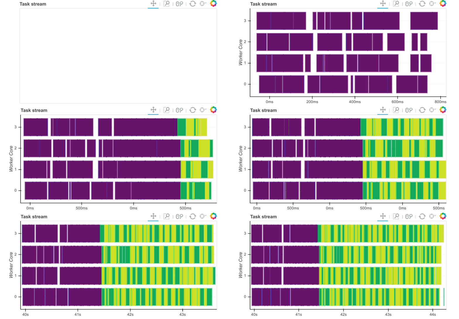
Now that we have the required data sets loaded and persisted in the database, let’s look at how fast this data can be extracted into Pandas and Dask dataframe objects as well as how fast certain trivial computation operations can be executed against those. Execution times are captured and visualised inside the notebook below using a simple matplotlib graph but Dask also comes with a nifty web interface to help deliver performance information over a standard web page in real time. This web interface is launched by default wherever the scheduler is launched providing the scheduler machine has Bokeh installed and includes data on system resources utilisation, tasks and workers progress, basic health checks etc. For example, the below task stream plot shows when tasks complete on which workers, with worker cores recorded on the y-axis and time on the x-axis.
For more detailed walkthrough of Dask web interface and its features Matthew Rocklin has a great video on YouTube – you can watch it HERE.
The below Jupyter notebook depicts sample Python code used to time the export of Sqlite data from 10 views created by the previous script visualised side by side for each view and library utilised (Pandas and Dask). It also compares execution times for some rudimentary operations e.g. sum(), max(), groupby() across three data sets i.e. 1 million, 5 million and 10 million records (again, read from Sqlite views). It is worth noting that Pandas, by design, is limited to a single CPU core execution (for most operations using standard CPython implementation thus being restricted by the Global Interpreter Lock GIL). Dask, on the other hand, was created from the ground-up to take advantage of multiple cores. By default, Dask Dataframe uses the multi-threaded scheduler. This exposes some parallelism when Pandas or the underlying NumPy operations release the global interpreter lock. Generally, Pandas is more GIL bound than NumPy, so multi-core speed-ups are not as pronounced for Dask DataFrame as they are for Dask Array. This is changing, and the Pandas development team is actively working on releasing the GIL. These few tests were run on my Mac Pro mid-2012 with 128GB DDR3 memory and dual Intel Xeon X5690 (12 cores/24 threads) CPUs. Dask version installed was v.1.2.2 and Python distribution version was v.3.6.8
Looking at the graph outlining comparative results between Dask and Pandas, it’s evident that data imports differ in performance and execution speed in favour of Dask. On the average, Dask seems to be twice as fast as Pandas when reading data from disk and this ratio is maintained across all data volumes in a fairly liner fashion.
Before I get to the computation performance overview, let’s look at how Dask utilised available resources to its advantage to parallelize number of operations across all available cores. All of the large-scale Dask collections like Dask Array, Dask DataFrame, and Dask Bag and the fine-grained APIs like delayed and futures generate task graphs where each node in the graph is a normal Python function and edges between nodes are normal Python objects that are created by one task as outputs and used as inputs in another task. After Dask generates these task graphs, it needs to execute them on parallel hardware. This is the job of a task scheduler. Different task schedulers exist, and each will consume a task graph and compute the same result, but with different performance characteristics. The threaded scheduler executes computations with a local multiprocessing.pool.ThreadPool. It is lightweight, requires no setup and it introduces very little task overhead (around 50us per task). Also, because everything occurs in the same process, it incurs no costs to transfer data between tasks. The threaded scheduler is the default choice for Dask Array, Dask DataFrame, and Dask Delayed. The below image captured CPU workload (using htop utility) during the below code execution. You can clearly see how Dask, by default, tried to spread the workload across multiple cores.
Looking at computation speed across number of different functions e.g. mean(), max(), groupby() the results are not as clear-cut as they were with the data import. Running these tests across three different data sources i.e. 1M, 5M and 10M records, Dask outperformed Pandas in ‘grouping’, ‘lambda’, ‘mean’ and ‘sum’ tests but surprisingly, in respect to ‘max’ and ‘min’, the advantage went to Pandas. I can only attribute this to the overhead Dask distributed scheduler creates when dispatching and collecting data across multiple threads/cores and Pandas efficiency in how it stores and indexes data inside the dataframe. Also, these datasets are quite small to truly do justice to how performant Dask can be in the right scenarios with the right environment setup and a lot more data to crunch so the old adage ‘the right tool for the right job’ is very fitting in this context.
To me it seems that Dask is more like a hammer, whereas Pandas is more akin to a scalpel – if you data is relatively small, Pandas is an excellent tool and the heavyweight approach of ‘divide and conquer’ is not the methodology you want to (or need to) use. Likewise, if your hardware and datasets are large enough to warrant taking advantage of parallelism and concurrency, Dask delivers on all fronts with minimal setup and API which is very similar to Pandas.
To sum up, the performance benefit (or drawback) of using a parallel dataframe like Dask dataframes over Pandas will differ based on the kinds of computations you do:
- If you’re doing small computations then Pandas is always the right choice. The administrative costs of parallelizing will outweigh any benefit. You should not parallelize if your computations are taking less than, say, 100ms.
- For simple operations like filtering, cleaning, and aggregating large data you should expect linear speedup by using a parallel dataframes. If you’re on a 20-core computer you might expect a 20x speedup. If you’re on a 1000-core cluster you might expect a 1000x speedup, assuming that you have a problem big enough to spread across 1000 cores. As you scale up administrative overhead will increase, so you should expect the speedup to decrease a bit.
- For complex operations like distributed joins it’s more complicated. You might get linear speedups like above, or you might even get slowdowns. Someone experienced in database-like computations and parallel computing can probably predict pretty well which computations will do well.




Never thought Polybase could be used in this capacity and don't think Microsoft advertised this feature (off-loading DB data as…