How To Build A Data Mart Using Microsoft BI Stack Part 7 – Cube Creation, Cube Deployment and Data Validation
In the PREVIOUS POST I showed you how to refine our SSAS project and went over the concepts of dimension properties and hierarchies before cube creation and deployment process can be initiated. In this post I would like to focus on the concepts of SSAS solution deployment and cube creation as well as go through some basic validation techniques to ensure that our data mart has correct data in it before it can be reported out of.
Creating The SSAS Cube
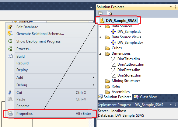
Let’s continue on with the sample SSAS project which we polished up last time. All files relevant to further develop, deploy and test this solution as well as all the code used in previous posts to this series can be found HERE. In order to browse the dimensions we must first deploy them to our SSAS database. Visual Studio uses XML files for data sources, data source views, dimensions, and cubes, and there is a hidden master file that contains all of this code. The act of building of an SSAS project checks the validity of these files and combines them into this master file. The quickest way to deploy is to it from Visual Studio environment itself, however, we must first specify the SSAS instance we would like our database to be created on. To do this, right-click on root level of the project in Solution Explorer and select Properties as per image below (Alt + Enter should also work).
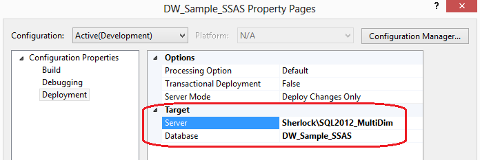
Next, select Deployment option from the Configuration Properties pane and populate the Target Server and Target Database as per below.
To process individual dimension we have meticulously created and deploy the data onto our SSAS server we can right-click on each dimension individually and select Process from the options provided. This should present us with another dialog window where providing we have done correct modelling decisions we can select Run to process our dimension. In case there are errors and you cannot deploy the data onto the specified SSAS server, go through the log to establish the cause for the issues which in most cases would pertain to the connection credentials or target deployment properties.
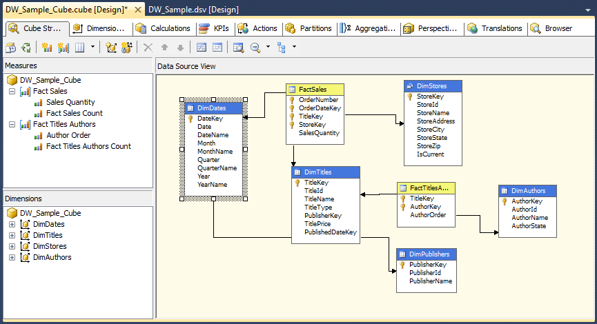
Finally, let’s look into how to create an SSAS cube. In order to start the cube wizard, right-click on the Cubes folder under solution explorer and select New Cube – this should start the wizard which will guide us through this process and is similar to the steps taken in order to create individual dimensions. After the welcome pane is displayed, click Next and on Select Creation Method click on Use Existing Tables from the options provided. Next step prompts us to select tables used for measure groups. This window allows you to choose which fact tables will be included in the cube. In our example, we have two fact tables: one that contains the measures and one that is used as a bridge between the Authors many-to-many dimension – let’s select them both and click next to continue with the wizard. In the next step, the wizard suggests columns and measures to use by comparing the columns’ data types. For example, Author Order is recommended as a measure because it is a fact table and it has a numeric value. This simple criteria is how the wizard decides what should and should not be included. You will also notice that Fact Sales Count and Fact Titles Authors Count have been added. The wizard suggests these additional measures to provide row counts for Fact Sales and Fact Titles Authors for your convenience, in case you need totals for each. The wizard labels these as Count measures for you, but you can change the names if you prefer. Following on, we select the four previously created dimensions and in the next step give our cube a meaningful name which should conclude the wizard. On completion Visual Studio displays cube designer window as per image below.
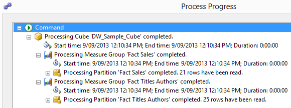
All there is left to do is to deploy the cube onto our server, configure it and test the data for any inconsistencies. The quickest way to deploy this is to right-click on the cube and select Process from the context menu provided. Once the process is completed, the following window should notify you of the process success/failure and the steps taken during cube processing and deployment.
There are other steps involved in further cube configuration which depends on the project requirements e.g. setting up translations, creating partitions, defining perspectives, adding custom calculations etc. however, given the intended purpose of this series I will not expand on those here. However, just like dimension, the cube also requires certain level of configuration input and validation so le’s run through those here.
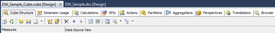
Most of the cube configuration is done through adjusting the settings on the cube designer tabs. Each of those tabs is responsible for different cube properties. The image below shows the tabs selection for cube designer.
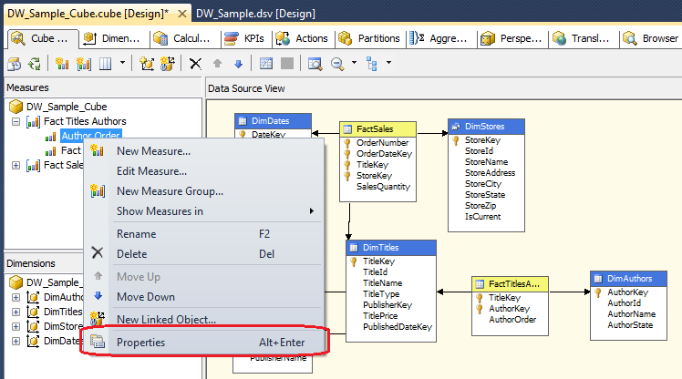
As far as configuring the properties of each measure and dimension which constitutes the cube content, these are usually accessed through the properties window on the Cube Structure tab. If you can’t see in it should be as easy as right-clicking on individual fact or dimension and selecting Properties from the context menu as per below.
To save space and leave the most procedural tasks out of this post I have put together a document which can be downloaded from HERE. It outlines the changes necessary to be made in order to configure the cube and its properties. Alternatively, you can view and download all the necessary files for this and other posts for this series from HERE.
Database vs. Cube Data Validation
Finally, let’s superficially validate the figures in the cube versus data warehouse objects to find out if what we have put together checks out and is a valid representation of our measures and dimensions. There are many very elaborate methods of validating the data between SSAS and database objects and in this post I will cover two ways of testing to highlight the potential discrepancies. The easiest way to compare the data between what’s in the cube and on the table level is to navigate to the Browser tab from the cube designer window (last tab) and drag desired measures and dimensions onto the query pane. This process is very much like building a pivot table in Excel and once the objects data is displayed and aggregated we can conveniently export the results into Excel straight from the SSAS project (version 2012 and up only) with a click of a button as per below.
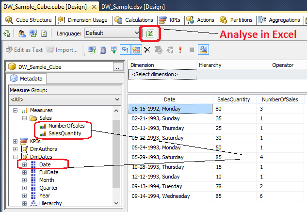
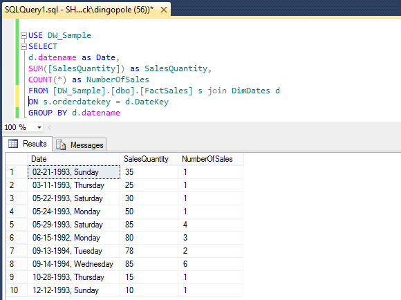
In the above image I dragged SalesQuantity and NumberOfSales measures as well as Date dimension onto the query pane and SSAS automatically aggregated the data for me. In order to validate that these figures are, in fact, what we store in the database let’s write a quick SQL and compare the output from both queries (even though the query can be composed by dragging and dropping measures/dimensions onto the query pane SSAS writes MDX code in the background).
USE DW_Sample
SELECT
d.datename as Date,
SUM([SalesQuantity]) as SalesQuantity,
COUNT(*) as NumberOfSales
FROM [DW_Sample].[dbo].[FactSales] s join DimDates d ON s.orderdatekey = d.DateKey
GROUP BY d.datename
When executed, the figures from the database which feeds out SSAS project are identical to those stored in the cube as per image below.
This method works well for small data sets but isn’t very effective with large volumes of data. Another, slightly more elaborate but also much more accurate and effective way is to create a linked server to our OLAP database and execute OPENQUERY SQL statement to extract the dimensional data in a tabular fashion for further comparison. First, let’s create a linked server executing the following SQL.
EXEC master.dbo.sp_addlinkedserver
@server = N'SQL2012_MultiDim',
@srvproduct = '',
@provider = N'MSOLAP',
@datasrc = N'Sherlock\sql2012_MultiDim',
@catalog = N'DW_Sample_SSAS'
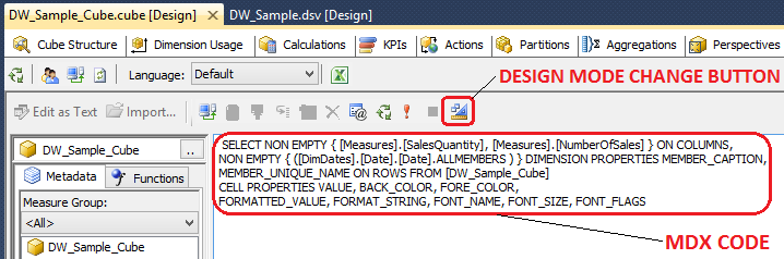
As you remember, when visually building a result set in a Browser tab in Visual Studio, SSAS also creates MDX code in the background. To access we simply click on the Design Mode button to change the interface from visual to code. If you had the desired result set already created visually, the MDX code should look similar to the one below.
Let’s copy the code and wrapping it around with an OPENQUERY SQL statement let’s bring back the results in Microsoft SQL Server Management Studio as per below.
SELECT *
FROM OPENQUERY
(SQL2012_MultiDim,
'SELECT NON EMPTY { [Measures].[SalesQuantity], [Measures].[NumberOfSales] } ON COLUMNS,
NON EMPTY { ([DimDates].[Date].[Date].ALLMEMBERS ) } DIMENSION PROPERTIES MEMBER_CAPTION,
MEMBER_UNIQUE_NAME ON ROWS FROM [DW_Sample_Cube]
CELL PROPERTIES VALUE, BACK_COLOR, FORE_COLOR,
FORMATTED_VALUE, FORMAT_STRING, FONT_NAME, FONT_SIZE, FONT_FLAGS')
Finally, after a little clean-up we can go ahead and compare the results between the cube and database using, for example, EXCEPT SQL statement as per the code snippet below.
SELECT
CAST("[DimDates].[Date].[Date].[Member_Caption]" AS nvarchar (50)) AS DateName,
CAST("[Measures].[SalesQuantity]" AS int) AS SalesQuantity,
CAST("[Measures].[NumberOfSales]" AS int) AS NumberOfSales
FROM OPENQUERY
(SQL2012_MultiDim,
'SELECT NON EMPTY { [Measures].[SalesQuantity], [Measures].[NumberOfSales] } ON COLUMNS,
NON EMPTY { ([DimDates].[Date].[Date].ALLMEMBERS ) } DIMENSION PROPERTIES MEMBER_CAPTION,
MEMBER_UNIQUE_NAME ON ROWS FROM [DW_Sample_Cube]
')

EXCEPT

SELECT
d.datename As DateName,
SUM([SalesQuantity]) as SalesQuantity,
COUNT(*) as SalesCount
FROM [DW_Sample].[dbo].[FactSales] s
join [DW_Sample].[dbo].[DimDates] d ON s.orderdatekey = d.DateKey
GROUP BY d.datename
If, after executing, the result brings back no values, this indicates data overlap and is symptomatic of that fact that there are no differences between the cube and the database. Similarly, you can try using INTERSECT SQL command in place if EXCEPT which should provide the opposite results i.e. only return the rows with identical data.
This concludes this post. As usual, the code used in this series as well as solution files for this SSAS project can be found and downloaded from HERE. In the NEXT ITERATION to the series I will be building a simple SSRS (SQL Server Reporting Services) report based on our data mart.
Please also check other posts from this series:
- How To Build A Data Mart Using Microsoft BI Stack Part 1 – Introduction And OLTP Database Analysis
- How To Build A Data Mart Using Microsoft BI Stack Part 2 – OLAP Database Objects Modelling
- How To Build A Data Mart Using Microsoft BI Stack Part 3 – Data Mart Load Approach And Coding
- How To Build A Data Mart Using Microsoft BI Stack Part 4 – Data Mart Load Using SSIS
- How To Build A Data Mart Using Microsoft BI Stack Part 5 – Defining SSAS Project And Its Dimensions
- How To Build A Data Mart Using Microsoft BI Stack Part 6 – Refining SSAS Data Warehouse Dimensions
- How To Build A Data Mart Using Microsoft BI Stack Part 8 – Creating Sample SSRS Report
All SQL code and solution files can be found and downloaded from HERE.
http://scuttle.org/bookmarks.php/pass?action=addThis entry was posted on Monday, September 16th, 2013 at 5:24 am and is filed under How To's, SQL, SSAS. You can follow any responses to this entry through the RSS 2.0 feed. You can leave a response, or trackback from your own site.


Hello Kind of what I've been looking for - thanks for posting. I don't use Snowflake but gives me an…