Snowflake Cloud Data Warehouse Review – TPC-DS Benchmark Performance Analysis and Why It’s Becoming the Post-Hadoop Big Data Nirvana

July 25th, 2020 / 20 Comments » / by admin

Note: All artifacts used in this demo can be downloaded from my shared OneDrive folder HERE.

Introduction

I have been working in the BI/Analytics field for a long time and have seen a lot of disruptive technologies in this space going through the hype cycle. Moving from SMP technologies to MPP databases, the era of Hadoop, the meteoric rise of Python and R for data science, serverless architectures and data lakes on cloud platforms etc. ensured that this industry stays more vibrant than ever. I see new frameworks, tools and paradigms raising to the surface almost daily and there are always new things to learn and explore. A few weeks ago, I had an interesting conversation with a recruiter about what’s trendy and interesting in the space of BI and Analytics and what the businesses she’s been helping with resourcing are looking for in terms of the IT talent pool. I was expecting to hear things like AI PaaS, Synthetic Data, Edge Analytics and all the interesting (and sometimes a bit over-hyped) stuff that the cool kids in Silicon Valley are getting into. Instead, she asserted that apart from public cloud platforms and all the run-of-the-mill BI tools like PowerBI and Looker, there is a growing demand for Snowflake projects. Mind you, this is an Australian market so chances are your neck of the woods may look completely different, but suffice to say, I didn’t expect a company not affiliated with a major public cloud provider to become so popular, particularly in this already congested market for cloud data warehousing solutions.

Snowflake, a direct competitor to Amazon’s Redshift, Microsoft’s Synapse and Google’s BigQuery, has been around for some time, but only recently I also started hearing more about it becoming the go-to technology for storing and processing large volumes of data in the cloud. I was also surprised to see Snowflake positioned in the ‘Leaders’ quadrant in the Data Management Solutions for Analytics chart, dethroning the well-known and respected industry stalwarts such as Vertica or Greenplum.

In this post, I want to look at Snowflake performance characteristics by creating a TPC-DS benchmark schema and executing a few analytical queries to see how it fares in comparison to some of the other MPP databases I worked with and/or tested. It’s not supposed to be an exhaustive overview or test and as such, these benchmark results should not be taken as Gospel. Having worked with databases all my career, I always look forward to exploring new technologies and even though I don’t expect to utilise Snowflake in my current project, it’s always exciting to kick the tires on a new platform or service.

OK, let’s dive in and see what’s in store!

Snowflake Architecture Primer

Snowflake claims to be built for cloud from the ground-up and does not offer on-premise deployment option, it’s purely a data warehouse as a service (DWaaS) offering. Everything – from database storage infrastructure to the compute resources used for analysis and optimisation of data – is handled by Snowflake. In this respect, Snowflake is not that much different from Google’s BigQuery although it’s difficult to contrast those two, mainly due to different pricing models (excluding storage cost) – BigQuery charges per volume of data scanned whereas Snowflake went with a more traditional model i.e. compute size and resource time allocation.

Snowflake’s architecture is a hybrid of traditional shared-disk database architectures and shared-nothing database architectures. Similar to shared-disk architectures, Snowflake uses a central data repository for persisted data that is accessible from all compute nodes in the data warehouse. But just like shared-nothing architectures, Snowflake processes queries using massively parallel processing compute clusters, where each node in the cluster stores a portion of the entire data set locally. This approach offers the data management simplicity of a shared-disk architecture, but with the performance and scale-out benefits of a shared-nothing architecture.

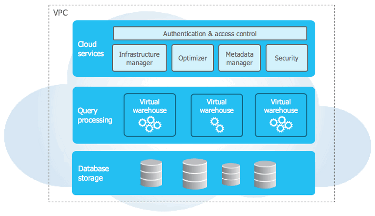
Snowflake’s unique architecture consists of three key layers:

  • Database Storage – When data is loaded into Snowflake, Snowflake reorganizes that data into its internaly optimized, compressed, columnar format. Snowflake stores this optimized data in cloud storage. Snowflake manages all aspects of how this data is stored — the organization, file size, structure, compression, metadata, statistics, and other aspects of data storage are handled by Snowflake. The data objects stored by Snowflake are not directly visible nor accessible by customers; they are only accessible through SQL query operations run using Snowflake
  • Query Processing – Query execution is performed in the processing layer. Snowflake processes queries using “virtual warehouses”. Each virtual warehouse is an MPP compute cluster composed of multiple compute nodes allocated by Snowflake from a cloud provider. Each virtual warehouse is an independent compute cluster that does not share compute resources with other virtual warehouses. As a result, each virtual warehouse has no impact on the performance of other virtual warehouses
  • Cloud Services – The cloud services layer is a collection of services that coordinate activities across Snowflake. These services tie together all of the different components of Snowflake in order to process user requests, from login to query dispatch. The cloud services layer also runs on compute instances provisioned by Snowflake from the cloud provider

Additionally, Snowflake can be hosted on any of the top three public cloud provides i.e. Azure, AWS and GCP across different regions, baring in mind that Snowflake accounts do not support multi-region deployments.

Loading TPC-DS Data

Data can be loaded into Snowflake is a number of ways, for example, using established ETL/ELT tools, using Snowpipe for continuous loading, WebUI or SnowSQL, and in a variety of formats e.g. JSON, AVRO, Parquet, CSV, Avro or XML. There are a few things to keep in mind when loading data into Snowflake which relate to file size, file splitting, file staging etc. The general recommendation is to produce files roughly 10MB to 100MB in size, compressed. Data loads of large Parquet files e.g. greater than 3GB could time out, therefore it is best practice to split those into smaller files to distribute the load among the servers in an active warehouse.

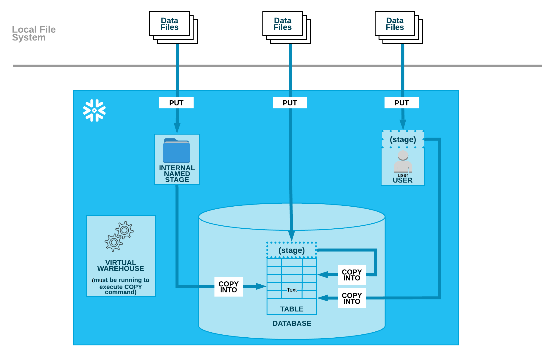
In order to run the TPC-DS queries on the Snowflake warehouse, I loaded the sample CSV-format data (scale factor of 100 and 300) from my local storage into the newly created schema using a small Python script. Snowflake also provides for staging files in public clouds object and blob storage e.g. AWS S3 but in this exercise, I transferred those from my local hard drive and staged them internally in Snowflake. As illustrated in the diagram below, loading data from a local file system is performed in two, separate steps:

  • Upload (i.e. stage) one or more data files to a Snowflake stage (named internal stage or table/user stage) using the PUT command
  • Use the COPY INTO command to load the contents of the staged file(s) into a Snowflake database table

As TPC-DS data does not conform to some of the requirements outlined above, the following script processed those files to ensure the format and size are consistent. The below script enables files format renaming (from DAT to CSV), breaking up larger files into smaller ones and removing trailing characters from line endings. It also creates the required TPC-DS schema and loads the pre-processed data into its objects.

#!/usr/bin/python
import snowflake.connector
from pathlib import PurePosixPath
import os
import re
import sys
from timeit import default_timer as timer, time
from humanfriendly import format_timespan
from csv import reader, writer
from multiprocessing import Pool, cpu_count


# define file storage locations variables
sql_schema = PurePosixPath("/Users/UserName/Location/SQL/tpc_ds_schema.sql")
tpc_ds_files_raw = PurePosixPath("/Volumes/VolumeName/Raw/")
tpc_ds_files_processed = PurePosixPath("/Volumes/VolumeName/Processed/")

# define other variables and their values
encoding = "iso-8859-1"
snow_conn_args = {
    "user": "username",
    "password": "password",
    "account": "account_name_on_a_public_cloud",
}
warehouse_name = "TPCDS_WH"
db_name = "TPCDS_DB"
schema_name = "tpc_ds"
output_name_template = "_%s.csv"
file_split_row_limit = 10000000


def get_sql(sql_schema):
    """
    Acquire sql ddl statements from a file stored in the sql_schema variable location
    """
    table_name = []
    query_sql = []

    with open(sql_schema, "r") as f:
        for i in f:
            if i.startswith("----"):
                i = i.replace("----", "")
                table_name.append(i.rstrip("\n"))

    temp_query_sql = []
    with open(sql_schema, "r") as f:
        for i in f:
            temp_query_sql.append(i)
        l = [i for i, s in enumerate(temp_query_sql) if "----" in s]
        l.append((len(temp_query_sql)))
        for first, second in zip(l, l[1:]):
            query_sql.append("".join(temp_query_sql[first:second]))
    sql = dict(zip(table_name, query_sql))
    return sql


def process_files(
    file,
    tpc_ds_files_raw,
    tpc_ds_files_processed,
    output_name_template,
    file_split_row_limit,
    encoding,
):
    """
    Clean up TPC-DS files (remove '|' row terminatinating characters)
    and break them up into smaller chunks in parallel
    """
    file_name = file[0]
    line_numer = 100000
    lines = []
    with open(
        os.path.join(tpc_ds_files_raw, file_name), "r", encoding=encoding
    ) as r, open(
        os.path.join(tpc_ds_files_processed, file_name), "w", encoding=encoding
    ) as w:
        for line in r:
            if line.endswith("|\n"):
                lines.append(line[:-2] + "\n")
                if len(lines) == line_numer:
                    w.writelines(lines)
                    lines = []
        w.writelines(lines)

    row_count = file[1]
    if row_count > file_split_row_limit:
        keep_headers = False
        delimiter = "|"
        file_handler = open(
            os.path.join(tpc_ds_files_processed, file_name), "r", encoding=encoding
        )
        csv_reader = reader(file_handler, delimiter=delimiter)
        current_piece = 1
        current_out_path = os.path.join(
            tpc_ds_files_processed,
            os.path.splitext(file_name)[0] +
            output_name_template % current_piece,
        )

        current_out_writer = writer(
            open(current_out_path, "w", encoding=encoding, newline=""),
            delimiter=delimiter,
        )
        current_limit = file_split_row_limit
        if keep_headers:
            headers = next(csv_reader)
            current_out_writer.writerow(headers)
        for i, row in enumerate(csv_reader):
            # pbar.update()
            if i + 1 > current_limit:
                current_piece += 1
                current_limit = file_split_row_limit * current_piece
                current_out_path = os.path.join(
                    tpc_ds_files_processed,
                    os.path.splitext(file_name)[0]
                    + output_name_template % current_piece,
                )
                current_out_writer = writer(
                    open(current_out_path, "w", encoding=encoding, newline=""),
                    delimiter=delimiter,
                )
                if keep_headers:
                    current_out_writer.writerow(headers)
            current_out_writer.writerow(row)
        file_handler.close()
        os.remove(os.path.join(tpc_ds_files_processed, file_name))


def build_schema(sql_schema, warehouse_name, db_name, schema_name, **snow_conn_args):
    """
    Build TPC-DS database schema based on the ddl sql returned from get_sql() function
    """
    with snowflake.connector.connect(**snow_conn_args) as conn:
        cs = conn.cursor()
        try:
            cs.execute("SELECT current_version()")
            one_row = cs.fetchone()
            if one_row:
                print("Building nominated warehouse, database and schema...")
                cs.execute("USE ROLE ACCOUNTADMIN;")
                cs.execute(
                    """CREATE OR REPLACE WAREHOUSE {wh} with WAREHOUSE_SIZE = SMALL 
                                                            AUTO_SUSPEND = 300 
                                                            AUTO_RESUME = TRUE 
                                                            INITIALLY_SUSPENDED = FALSE;""".format(
                        wh=warehouse_name
                    )
                )
                cs.execute("USE WAREHOUSE {wh};".format(wh=warehouse_name))
                cs.execute(
                    "CREATE OR REPLACE DATABASE {db};".format(db=db_name))
                cs.execute("USE DATABASE {db};".format(db=db_name))
                cs.execute(
                    "CREATE OR REPLACE SCHEMA {sch};".format(sch=schema_name))
                sql = get_sql(sql_schema)
                for k, v in sql.items():
                    try:
                        k = k.split()[-1]
                        cs.execute(
                            "drop table if exists {sch}.{tbl};".format(
                                sch=schema_name, tbl=k
                            )
                        )
                        cs.execute(v)
                    except Exception as e:
                        print(e)
                        print("Error while creating nominated database object", e)
                        sys.exit(1)
        except (Exception, snowflake.connector.errors.ProgrammingError) as error:
            print("Could not connect to the nominated snowflake warehouse.", error)
        finally:
            cs.close()


def load_data(encoding, schema_name, db_name, tpc_ds_files_processed, **snow_conn_args):
    """
    Create internal Snowflake staging area and load csv files into Snowflake schema
    """
    stage_name = "tpc_ds_stage"
    paths = [f.path for f in os.scandir(tpc_ds_files_processed) if f.is_file()]
    with snowflake.connector.connect(**snow_conn_args) as conn:
        cs = conn.cursor()
        cs.execute("USE ROLE ACCOUNTADMIN;")
        cs.execute("USE WAREHOUSE {wh};".format(wh=warehouse_name))
        cs.execute("USE DATABASE {db};".format(db=db_name))
        cs.execute("USE SCHEMA {sch};".format(sch=schema_name))
        cs.execute("drop stage if exists {st};".format(st=stage_name))
        cs.execute(
            """create stage {st} file_format = (TYPE = "csv" 
                                FIELD_DELIMITER = "|" 
                                RECORD_DELIMITER = "\\n")
                                SKIP_HEADER = 0 
                                FIELD_OPTIONALLY_ENCLOSED_BY = "NONE" 
                                TRIM_SPACE = FALSE 
                                ERROR_ON_COLUMN_COUNT_MISMATCH = TRUE 
                                ESCAPE = "NONE" 
                                ESCAPE_UNENCLOSED_FIELD = "\\134" 
                                DATE_FORMAT = "AUTO" 
                                TIMESTAMP_FORMAT = "AUTO" 
                                NULL_IF = ("NULL")""".format(
                st=stage_name
            )
        )
        for path in paths:
            try:
                file_row_rounts = sum(
                    1
                    for line in open(
                        PurePosixPath(path), "r+", encoding="iso-8859-1", newline=""
                    )
                )
                file_name = os.path.basename(path)
                # table_name = file_name[:-4]
                table_name = re.sub(r"_\d+", "", file_name[:-4])
                cs.execute(
                    "TRUNCATE TABLE IF EXISTS {tbl_name};".format(
                        tbl_name=table_name)
                )
                print(
                    "Loading {file_name} file...".format(file_name=file_name),
                    end="",
                    flush=True,
                )
                sql = (
                    "PUT file://"
                    + path
                    + " @{st} auto_compress=true".format(st=stage_name)
                )
                start = timer()
                cs.execute(sql)
                sql = (
                    'copy into {tbl_name} from @{st}/{f_name}.gz file_format = (ENCODING ="iso-8859-1" TYPE = "csv" FIELD_DELIMITER = "|")'
                    ' ON_ERROR = "ABORT_STATEMENT" '.format(
                        tbl_name=table_name, st=stage_name, f_name=file_name
                    )
                )
                cs.execute(sql)
                end = timer()
                time = round(end - start, 1)
                db_row_counts = cs.execute(
                    """SELECT COUNT(1) FROM {tbl}""".format(tbl=table_name)
                ).fetchone()
            except (Exception, snowflake.connector.errors.ProgrammingError) as error:
                print(error)
                sys.exit(1)
            finally:
                if file_row_rounts != db_row_counts[0]:
                    raise Exception(
                        "Table {tbl} failed to load correctly as record counts do not match: flat file: {ff_ct} vs database: {db_ct}.\
                            Please troubleshoot!".format(
                            tbl=table_name,
                            ff_ct=file_row_rounts,
                            db_ct=db_row_counts[0],
                        )
                    )
                else:
                    print("OK...loaded in {t}.".format(
                        t=format_timespan(time)))


def main(
    sql_schema,
    warehouse_name,
    db_name,
    schema_name,
    tpc_ds_files_raw,
    tpc_ds_files_processed,
    output_name_template,
    file_split_row_limit,
    encoding,
    **snow_conn_args
):
    """
    Rename TPC-DS files, do a row count for each file to determine the number of smaller files larger ones need to be split into 
    and kick off parallel files cleanup and split process. Finally, kick off schema built and data load into Snowflake
    """
    for file in os.listdir(tpc_ds_files_raw):
        if file.endswith(".dat"):
            os.rename(
                os.path.join(tpc_ds_files_raw, file),
                os.path.join(tpc_ds_files_raw, file[:-4] + ".csv"),
            )
    fileRowCounts = []
    for file in os.listdir(tpc_ds_files_raw):
        if file.endswith(".csv"):
            fileRowCounts.append(
                [
                    file,
                    sum(
                        1
                        for line in open(
                            os.path.join(tpc_ds_files_raw, file),
                            encoding=encoding,
                            newline="",
                        )
                    ),
                ]
            )
    p = Pool(processes=cpu_count())
    for file in fileRowCounts:
        p.apply_async(
            process_files,
            [
                file,
                tpc_ds_files_raw,
                tpc_ds_files_processed,
                output_name_template,
                file_split_row_limit,
                encoding,
            ],
        )
    p.close()
    p.join()
    build_schema(sql_schema, warehouse_name, db_name,
                 schema_name, **snow_conn_args)
    load_data(encoding, schema_name, db_name,
              tpc_ds_files_processed, **snow_conn_args)


if __name__ == "__main__":
    main(
        sql_schema,
        warehouse_name,
        db_name,
        schema_name,
        tpc_ds_files_raw,
        tpc_ds_files_processed,
        output_name_template,
        file_split_row_limit,
        encoding,
        **snow_conn_args
    )

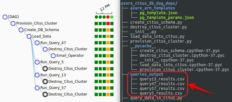
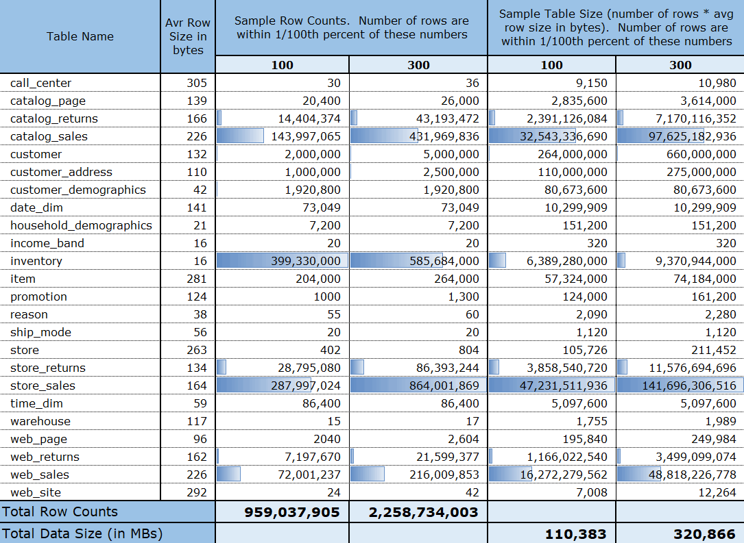
Once executed, the script produced 246 CSV files (up from 26 in the original data set) and on load completion, the following data volume (uncompressed) and row count metadata was created in Snowflake warehouse.

TPC-DS Benchmark Sample

Although Snowflake conveniently provides 10TB and 100TB versions of TPC-DS data, along with samples of all the benchmark’s 99 queries, I really wanted to go through the whole process myself to help me understand the service and tooling it provides in more details. In hindsight, it turned out to be an exercise in patience thanks to my ISP’s dismal upload speed so if you’re looking at kicking the tires and simply running a few queries yourself, it may be quicker to use Snowflake’s provided data sets.

It is worth mentioning that no performance optimisation was performed on the queries, data or system itself. Unlike other vendors which allows their administrators to fine-tune various aspects of its operation through mechanisms such as statistics update, table partitioning, creating query or workload-specific projections, tuning execution plans etc. Snowflake obfuscates a lot of those details away. Beyond elastically scaling compute down or up or defining cluster key to help with execution on very large tables, there is very little knobs and switches one can play with. That’s a good thing and unless you’re a consultant making money helping your clients with performance tuning, many engineers will be happy to jump on the bandwagon for this reason alone.

Also, data volumes analysed in this scenario do not follow the characteristics and requirements outline by the TPC organisation and under these circumstances would be considered an ‘unacceptable consideration’. For example, a typical benchmark submitted by a vendor needs to include a number of metrics beyond query throughput e.g. a price-performance ratio, data load times, the availability date of the complete configuration etc. The following is a sample of a compliant reporting of TPC-DS results: ‘At 10GB the RALF/3000 Server has a TPC-DS Query-per-Hour metric of 3010 when run against a 10GB database yielding a TPC-DS Price/Performance of $1,202 per query-per-hour and will be available 1-Apr-06’. As this demo and the results below go only skin-deep i.e. query execution times, the results are only indicative of the performance level in the context of the same data and configuration used.

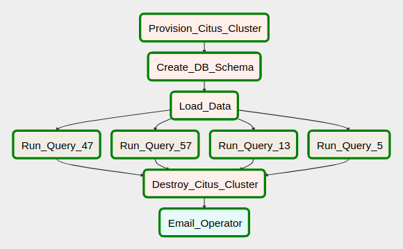
OK, now with this little declaimer out of the way let’s look at how the 24 queries performed across the two distinct setups i.e. a Small warehouse and a Large warehouse across 100GB and 300GB datasets. I used the following Python script to return queries execution time.

#!/usr/bin/python
import configparser
import sys
from os import path, remove
from pathlib import PurePosixPath
import snowflake.connector
from timeit import default_timer as timer
from humanfriendly import format_timespan

db_name = "TPCDS_DB"
schema_name = "tpc_ds"
warehouse_name = "TPCDS_WH"
snow_conn_args = {
    "user": "username",
    "password": "password",
    "account": "account_name_on_a_public_cloud",
}

sql_queries = PurePosixPath(
    "/Users/UserName/Location/SQL/tpc_ds_sql_queries.sql"
)


def get_sql(sql_queries):
    """
    Source operation types from the tpc_ds_sql_queries.sql SQL file.
    Each operation is denoted by the use of four dash characters 
    and a corresponding query number and store them in a dictionary 
    (referenced in the main() function). 
    """
    query_number = []
    query_sql = []

    with open(sql_queries, "r") as f:
        for i in f:
            if i.startswith("----"):
                i = i.replace("----", "")
                query_number.append(i.rstrip("\n"))

    temp_query_sql = []
    with open(sql_queries, "r") as f:
        for i in f:
            temp_query_sql.append(i)
        l = [i for i, s in enumerate(temp_query_sql) if "----" in s]
        l.append((len(temp_query_sql)))
        for first, second in zip(l, l[1:]):
            query_sql.append("".join(temp_query_sql[first:second]))
    sql = dict(zip(query_number, query_sql))
    return sql


def run_sql(
    query_sql, query_number, warehouse_name, db_name, schema_name
):
    """
    Execute SQL query as per the SQL text stored in the tpc_ds_sql_queries.sql
    file by it's number e.g. 10, 24 etc. and report returned row number and 
    query processing time
    """
    with snowflake.connector.connect(**snow_conn_args) as conn:
        try:
            cs = conn.cursor()
            cs.execute("USE ROLE ACCOUNTADMIN;")
            cs.execute("USE WAREHOUSE {wh};".format(wh=warehouse_name))
            cs.execute("USE DATABASE {db};".format(db=db_name))
            cs.execute("USE SCHEMA {sch};".format(sch=schema_name))
            query_start_time = timer()
            rows = cs.execute(query_sql)
            rows_count = sum(1 for row in rows)
            query_end_time = timer()
            query_duration = query_end_time - query_start_time
            print(
                "Query {q_number} executed in {time}...{ct} rows returned.".format(
                    q_number=query_number,
                    time=format_timespan(query_duration),
                    ct=rows_count,
                )
            )
        except (Exception, snowflake.connector.errors.ProgrammingError) as error:
            print(error)
        finally:
            cs.close()


def main(param, sql):
    """
    Depending on the argv value i.e. query number or 'all' value, execute 
    sql queries by calling run_sql() function
    """
    if param == "all":
        for key, val in sql.items():
            query_sql = val
            query_number = key.replace("Query", "")
            run_sql(
                query_sql,
                query_number,
                warehouse_name,
                db_name,
                schema_name
            )
    else:
        query_sql = sql.get("Query" + str(param))
        query_number = param
        run_sql(
            query_sql,
            query_number,
            warehouse_name,
            db_name,
            schema_name
        )


if __name__ == "__main__":
    if len(sys.argv[1:]) == 1:
        sql = get_sql(sql_queries)
        param = sys.argv[1]
        query_numbers = [q.replace("Query", "") for q in sql]
        query_numbers.append("all")
        if param not in query_numbers:
            raise ValueError(
                "Incorrect argument given. Looking for <all> or <query number>. Specify <all> argument or choose from the following numbers:\n {q}".format(
                    q=", ".join(query_numbers[:-1])
                )
            )
        else:
            param = sys.argv[1]
            main(param, sql)
    else:
        raise ValueError(
            "Too many arguments given. Looking for 'all' or <query number>."
        )

First up is the 100GB dataset, with queries running on empty cache (cached results were sub-second therefore I did not bother to graph those here), across Small and Large warehouses. When transitioning from the Small to the Large warehouse, I also dropped the existing warehouse (rather than resizing it), created a new one and re-populated it to ensure that not data is returned from cache.

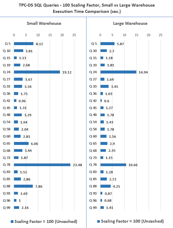
While these results and test cases are probably not truly representative of the ‘big data’ workloads, they provide a quick snapshot of how traditional analytical workloads would perform on the Snowflake platform. Scanning large tables with hundreds of millions of rows seemed to perform quite well, and, for the most part, performance differences were consistent with the increase in compute capacity. Cached queries run nearly instantaneously so looking at the execution pattern for cached vs non-cached results there was contest (and no point in comparing and graphing the results). Interestingly, I did a similar comparison for Google’s BigQuery platform (link HERE) and Snowflake seems to perform a lot better in this regard i.e. cached results are returned with low latency, usually in less than one second. Next up I graphed the 300GB scaling factor, again repeating the same queries across Small and Large warehouse size.

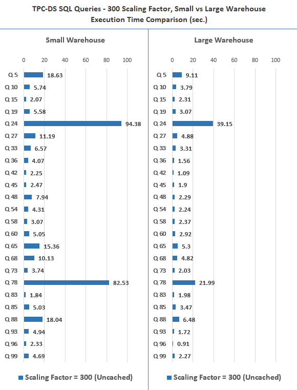
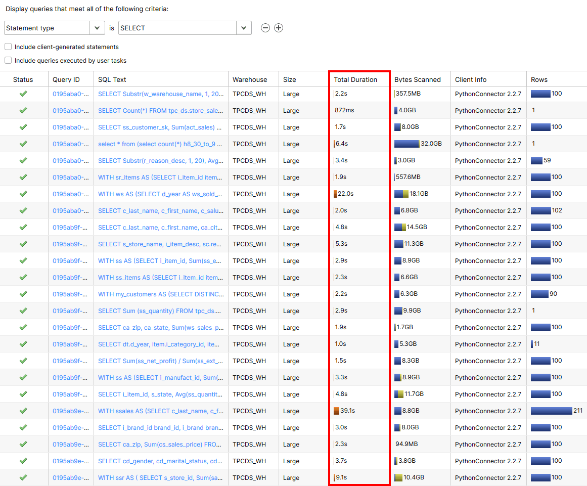
Snowflake’s performance on the 300GB dataset was very good and majority of the queries returned relatively fast. Side by side, it is easy to see the difference the larger compute allocation made to queries’ execution time, albeit at the cost of increased credits usage. Current pricing model dictates that Large warehouse is 4 times as expensive as a Small one. Given the price of a credit (standard, single-cluster warehouse) in AWS Sydney region is currently set to USD 2.75, 22 dollars per hour for the Large warehouse (not including storage and cloud services cost), it becomes a steep proposition at close to AUD 100K/year (assuming that only 12/24 hours will be charged and only during work days). Cost notwithstanding, Snowflake is a powerful platform and the ability to crunch a lot of data at this speed and on demand is commendable. Although a bit of an apples-to-oranges comparison, you can also view how BigQuery performed on exactly identical datasets in one of my previous posts HERE. Also, just for reference, I below is an image of metadata maintained by Snowflake itself on all activities across the warehouse, filtered to display only SELECT statements information (un-cached 300GB Large warehouse run in this case).

Snowflake Reference Architectures

What I’m currently seeing in the industry from the big data architecture patterns point of view is that business tend to move towards deployments favored by either data engineering teams or BI/Analytics teams. The distinction across those two groups is heavily determined by the area of expertise and the tooling used, with DE shops more reliant on software engineering paradigms and BI folks skills skewed more towards SQL for most of their data processing needs. This allows teams not versed in software development to use vanilla SQL to provision and manage most of their data-related responsibilities and therefore Snowflake to effectively replace development-heavy tasks with the simplicity of its platform. Looking at what an junior analyst can achieve with just a few lines of SQL in Snowflake allows many businesses to drastically simplify and, at the same time, supercharge their analytical capability, all without the knowledge of programming in Scala or Python, distributed systems architecture, bespoke ETL frameworks or intricate cloud concepts knowledge. In the past, a plethora of tools and platforms would be required to shore up analytics pipelines and workloads. With Snowflake, many of those e.g. traditional, files-based data lakes, semi-structured data stores etc. can become redundant, with Snowflake becoming the linchpin of the enterprise information architecture.

The following are some examples of reference architectures used across several use cases e.g. IoT, streaming data stack, ML and data science, demonstrating Snowflake’s capabilities in supporting those varied scenarios with their platform.

Conclusion

Data warehousing realm has been dominated by a few formidable juggernauts of this industry and no business outside of few start-ups would be willing to bet their data on an up-and-coming entrant who is yet to prove itself. A few have tried but just as public cloud space is starting to consolidate and winners take it all, data warehousing domain has always been difficult to disrupt. In the ever-expanding era of cloud computing, many vendors are rushing to retool and retrofit their existing offering to take advantage of this new paradigm, but ultimately few offer innovative and fresh approaches. Starting from the ground-up and with no legacy and technical debt to worry about, Snowflake clearly is trying to reinvent the approach and I have to admit I was quite surprised by not only how well Snowflake performed in my small number of tests but also how coherent the vision is. They are not trying to position themselves as the one-stop-shop for ETL, visualisation and data warehousing. There is no mention of running their workloads on GPUs or FPGAs, no reference to Machine Learning or AI (not yet anyway) and on the face value, the product is just a reinvented data warehouse cloud appliance. Some may consider it a shortcoming as integration with other platforms, services and tools (something that Microsoft and AWS are doing so well) may be a paramount criterion. However, this focus on ensuring that the one domain they’re targeting gets the best engineering in its class is clearly evident. Being Jack of all trades and master of none may work for the Big Cheese so Snowflake is clearly trying to come up with a superior product in a single vertical and not devalue their value proposition – something that they have been able to excel at so far.

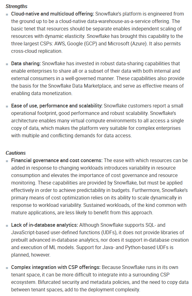
After nearly 15 years of working in the information management field and countless encounters with different vendors, RDBMSs, platforms etc. Snowflake seems like a breath of fresh air to me. It supports a raft of different connectors and drivers, speaks plain SQL, is multi-cloud, separates storage from compute, scales automatically, requires little to no tuning and performs well. It also comes with some great feature built-in, something that in case of other vendors may require a lot of configuration, expensive upgrades or even bespoke development e.g. time travel, zero-copy cloning, materialized views, data sharing or continuous data loading using Snowpipe. On the other hand, there are a few issues which may become a deal-breaker for some. A selection of features is only available in the higher (more expensive) tiers e.g. time travel or column-level security, there is no support for constraints and JavaScript-based UDFs/stored procedures are a pain to use. The Web UI is clean but a bit bare-bones and integration with some of the legacy tools may prove to be challenging. Additionally, the sheer fact that you’re not in control of the infrastructure and data (some industries are still limited to how and where their data is stored) may turn some interested parties away, especially that MPP engines like Greenplum, Vertica or ClickHouse can be deployed on both private and public clouds. Below is an excerpt from 2020 Gartner Magic Quadrant for Cloud Database Management Systems, outlining Snowflake’s core strengths and weaknesses.

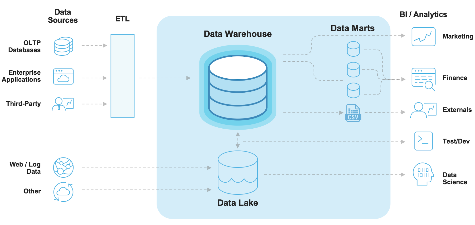
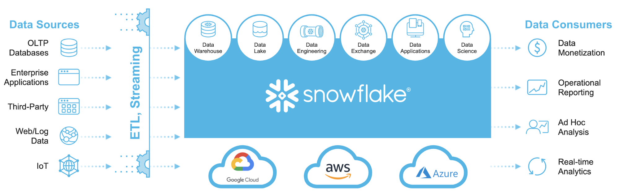
What I personally liked the most about this service is how familiar and simple it is, while providing all required features in a little to no-ops package. I liked the fact that in spite of all the novel architecture it’s built on, it feels just like another RDBMS. If I could compare it to a physical thing, it would be a (semi)autonomous electric car. Just like any automobile, EVs sport four wheels, lights, doors and everything else that unmistakably make them a vehicle. Likewise, Snowflake speaks SQL (a 40 years old language), has tables, views, UDFs and has all the features traditional databases have had for decades. However, just as the new breed of autonomous cars don’t come with a manual transmission, gas-powered engines, detailed mechanical service requirements or even a steering wheel, Snowflake looks to be built for the future, blending old-school familiarity and pioneering technology together. It is no-fuss, low-ops, security-built-in, cloud-only service which feels instantaneously recognizable and innovative at the same time. It’s not your grandpa’s data warehouse and, in my view, it has nearly all the features to rejuvenate and simplify a lot of the traditional BI architectures. The following is a comparison of a traditional vs contemporary data warehouse architectures, elevating Snowflake to the centerpiece of the data storage and processing platform.

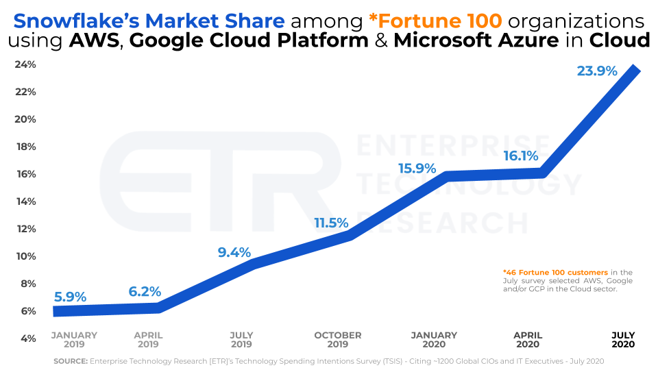
Many vendors are rushing to adapt and transform their on-premise-first data warehouse software with varied success. Oracle, IBM or Microsoft come to mind when looking at a popular RDBMSs engines running predominantly in customers’ data centers. All of those vendors are now pushing hard to customize their legacy products and ensure that the new iteration of their software is cloud-first but existing technical debt and the scope of investment already made may create unbreakable shackles, stifling innovation and compromising progress. Snowflake’s new approach to solving data management problems has gained quite a following and many companies are jumping on board in spite the fact that they are not affiliated with any of the major cloud vendors and the competition is rife – only last week Google announced BigQuery Omni. Looking at one of the most recent Data Warehouse market analysis (source HERE), Snowflake has been making some serious headway among Fortune 100 companies and is quickly capitalizing on its popularity and accelerating adoption rate. The chart below is a clear evidence of this and does not require any explanation – Snowflake is on a huge roll.

It’s still early days and time will tell if Snowflake can maintain the momentum but having spent a little time with it, I understand the appeal and why their service is gaining in popularity. If I was looking at storing and processing large volume of data and best of breed data warehousing capability, Snowflake would definitely be on my shopping list.

Tags: , , , , , ,

Kicking the Tires on Airflow, Apache’s workflow management platform – Architecture Overview, Installation and sample Azure Cloud Deployment Pipeline in Python (Part 2)

May 24th, 2020 / 4 Comments » / by admin

Airflow Sample Workflow Continued…

Note: Part 1 can be found HERE and all files used in this tutorial can be downloaded from HERE.

In the first part to this short series on Apache Airflow I outlined it its core architecture, installation process and created a sample example of a very rudimentary DAG (Directed Acyclic Graph). In this post I’d like to dive a bit deeper and look at a more advanced workflow which combines a few different operations and tasks. Let’s assume that we’re tasked with creating a DAG which needs to accomplish the following:

  • Programmatically create Citus database instance in Azure public cloud with specific configuration parameters e.g. geographic location, storage size, number of nodes assigned, firewall rules etc. These parameters are stored across two JSON template files, known Azure Resource Manager templates
  • Subsequently to creating Azure Citus database, the workflow should create a database schema using DDL SQL stored in one of the configuration files
  • Next, load text files data into the newly created database schema
  • Run four sample TPC-DS SQL queries in parallel (queries 5, 13, 47 and 57) and store the results into a file on the local file system
  • Shut the cluster down and remove any resources created as part of this process
  • Send out an e-mail notifying operator(s) of the workflow conclusion

A similar type of workload is often used to create an idempotent pipeline which stitches together a number of tasks, including cloud infrastructure provisioning, data analytics, ETL/ELT activities etc. to design an end-to-end data management solution. The required DAG, with all its dependencies and activities should like as per the image below.

Sample Airflow Azure Cloud Pipeline Architecture

In order to provision the Azure resource groups and resources, I have created two JSON template files, also known as Azure Resource Manager (ARM) templates, which contain the required resources and their properties. ARM templates allow for declarative creation and deployment of any Azure infrastructure components e.g. virtual machines, hosted databases, storage accounts etc. along their properties and names. As the libraries used in the Python version of the Azure SDK directly mirror and consume Azure service’s REST endpoints, it’s quite easy to script out a repeatable deployment process using ARM templates as described in more details further along in this post. As part of the solution configuration, I have also created two SQL files which are used to create a suite of tables on the Citus cluster and run the queries, outputting the result sets into a local directory.

The aforementioned files used to populate the Citus cluster schema are part of the TPC-DS benchmark data (scaling factor set to 1GB) and consist of a number of flat files in a CSV format. As we’re not going to recreate the whole TPC-DS benchmark suite of tests (this post is not intended to evaluate Citus database performance), to simplify the data loading process, I will only use a few of them (just over 800MB in size), which should provide us with enough data to run a few queries once the tables have been populated. To simplify this demonstration, all Python solution files as well as ARM JSON templates, SQL files and flat files data were moved into dags directory aka {AIRFLOW_HOME}/dags folder. Under typical scenario, data would not co-exists with configuration and solution files but for this exercise, I have nominated to structure the project as per the the directory breakdown on the left. Also, in a production environment, particularly one with many dag and task files, you would want to ensure that a consistent organizational structure is imposed across DAG folder and its sub-directories. As Airflow is such a versatile tool, depending on a specific use case, you may want to separate individual projects and their related hooks, operators, scripts and other files into their own respective folders etc.

With Airflow server up and running (installation and configuration instructions in the previous post HERE) and the files required to load into our Citus database schema staged in the solution directory we can start unpacking individual code samples used in the final DAG. As mentioned at the start, Citus database cluster, just as any other Azure resource, can be spun up declaratively using ARM template(s). You can peruse the content of the templates used in this demo as well as other artifacts in my publicly accessible OneDrive folder HERE.

A quick word about Citus (now owned by Microsoft). Citus is an open source extension to PostgreSQL which distributes data and queries across multiple nodes. Because Citus is an extension to PostgreSQL (not a fork), it gives developers and enterprises a scale-out database while keeping the power and familiarity of a relational database. Citus horizontally scales PostgreSQL across multiple machines using sharding and replication. Its query engine parallelizes incoming SQL queries across these servers to enable super-fast responses on even very large datasets. I’m not very familiar with the service but there are many posts on the Internet describing some interesting projects Citus was used in, beating other competing technologies (TiDB, Apache Pinot, Apache Kylin, Apache Druid), partly due to its great SQL support and a large community of PostgreSQL users who are already familiar with the RDBMS it is based on e.g. HERE.

Now, let’s go through the individual scripts and unpack the whole solution piece by piece. The following Python script is using ARM templates to provision Azure resource group and a small Citus database cluster (single coordinator node and two worker nodes).

import adal
from timeit import default_timer as timer
from sys import platform
from msrestazure.azure_active_directory import AdalAuthentication
from msrestazure.azure_cloud import AZURE_PUBLIC_CLOUD
from azure.mgmt.resource.resources.models import (
    DeploymentMode,
    DeploymentProperties,
    Deployment,
)
from azure.mgmt.resource import ResourceManagementClient
from pathlib import Path, PurePosixPath
import json
import os

arm_template_location = PurePosixPath(
    "/home/airflow/airflow/dags/azure_citus_db_dag_deps/azure_arm_templates/pg_template.json"
)
arm_template_params_location = PurePosixPath(
    "/home/airflow/airflow/dags/azure_citus_db_dag_deps/azure_arm_templates/pg_template_params.json"
)

resource_group = "citus_svr_resource_group"
external_IP = os.popen("curl -s ifconfig.me").readline()
deployment_name = "azure_citus_deployment"

external_ip_params = {
    "name": "ClientIPAddress",
    "startIPAddress": external_IP,
    "endIPAddress": external_IP,
}
admin_login = {"value": "citus"}
admin_passwd = {"value": "your_citus_password"}

template = arm_template_location
params = arm_template_params_location

if template:
    with open(template, "r") as json_file_template:
        template = json.load(json_file_template)

if params:
    with open(params, "r") as json_file_template:
        params = json.load(json_file_template)
        params = {k: v for k, v in params["parameters"].items()}
        params["firewallRules"]["value"]["rules"][1] = external_ip_params
        params["administratorLogin"] = admin_login
        params["administratorLoginPassword"] = admin_passwd
        resource_group_location = params["location"]["value"]


# Tenant ID for your Azure Subscription
TENANT_ID = "123a27e2-7777-4d30-9ca2-ce960d430ef8"

# Your Service Principal App ID
CLIENT = "ae277f4e-882d-4f03-a0b5-b69275046123"

# Your Service Principal Password
KEY = "e7bbf0ed-d461-48c7-aace-c6a4822a123e"

# Your Azure Subscription ID
subscription_id = "1236a74c-dfd8-4b4d-b0b9-a355d2ec793e"

LOGIN_ENDPOINT = AZURE_PUBLIC_CLOUD.endpoints.active_directory
RESOURCE = AZURE_PUBLIC_CLOUD.endpoints.active_directory_resource_id

context = adal.AuthenticationContext(LOGIN_ENDPOINT + "/" + TENANT_ID)
credentials = AdalAuthentication(
    context.acquire_token_with_client_credentials, RESOURCE, CLIENT, KEY
)

client = ResourceManagementClient(credentials, subscription_id)


def create_citus_instance(resource_group):

    deployment_properties = {
        "mode": DeploymentMode.incremental,
        "template": template,
        "parameters": params,
    }

    deployment_async_operation = client.deployments.create_or_update(
        resource_group, deployment_name, deployment_properties
    )

    deployment_async_operation.wait()


def main():
    print("\nCreating Azure Resource Group...")
    start = timer()
    client.resource_groups.create_or_update(
        resource_group, {"location": resource_group_location}
    )
    print("Creating Citus Cluster...")
    create_citus_instance(resource_group)
    end = timer()
    time = round(end - start, 1)
    print("Total Elapsed Deployment Time = {t} seconds".format(
        t=format(time, ".2f")))


if __name__ == "__main__":
    main()

This file, called provision_citus_cluster.py, will be called from our Airflow DAG using PythonOperator and is the first step of our pipeline. The instance creation process should take a few minutes to provision and once created we can continue on and generate Citus cluster schema with all the required objects.

In order to populate Citus database with the flat files data we first need to create the desired schema (in this case called tpc_ds) and all the required objects. Even though this process will not be populating all tables (there are only thirteen flat files to be loaded), the script will create all TPC-DS benchmark objects using a simple SQL file containing all necessary DDL statements. The actual SQL file can be viewed and downloaded from my OneDrive folder so to keep this post concise, I will only include the Python script which parses the DDL SQL statements and executes those, creating all required tables. This operation (called from create_citus_schema.py file) will generate a second object in our DAG’s chain of tasks.

from pathlib import Path, PurePosixPath
from sys import platform
from psycopg2.extensions import ISOLATION_LEVEL_AUTOCOMMIT
import psycopg2
import sys

sql_schema = PurePosixPath(
    "/home/airflow/airflow/dags/azure_citus_db_dag_deps/sql/tpc_ds_schema.sql"
)

pg_args = {
    "user": "citus",
    "password": "your_citus_password",
    "host": "citussvrgroup-c.postgres.database.azure.com",
    "port": "5432",
    "database": "citus",
    "sslmode": "require",
}

pg_schema_name = "tpc_ds"


def get_sql(sql_schema):
    """
    Source operation types from the 'create_sqlite_schema' SQL file.
    Each operation is denoted by the use of four dash characters
    and a corresponding table DDL statement and store them in a dictionary
    (referenced in the main() function).
    """
    table_name = []
    query_sql = []

    with open(sql_schema, "r") as f:
        for i in f:
            if i.startswith("----"):
                i = i.replace("----", "")
                table_name.append(i.rstrip("\n"))

    temp_query_sql = []
    with open(sql_schema, "r") as f:
        for i in f:
            temp_query_sql.append(i)
        l = [i for i, s in enumerate(temp_query_sql) if "----" in s]
        l.append((len(temp_query_sql)))
        for first, second in zip(l, l[1:]):
            query_sql.append("".join(temp_query_sql[first:second]))
    sql = dict(zip(table_name, query_sql))
    return sql


def build_schema(sql_schema, pg_schema_name, **kwargs):
    connection = None
    try:
        connection = psycopg2.connect(**kwargs)
        cursor = connection.cursor()
        cursor.execute("SELECT version();")
        record = cursor.fetchone()
        if record:
            connection.set_isolation_level(ISOLATION_LEVEL_AUTOCOMMIT)
            cursor.execute(
                "CREATE SCHEMA IF NOT EXISTS {s};".format(
                    s=pg_schema_name)
            )
            conn_params = connection.get_dsn_parameters()
            if conn_params["dbname"] == "citus":
                sql = get_sql(sql_schema)
                ddls = sql.values()
                for s in ddls:
                    try:
                        cursor.execute(s)
                        connection.commit()
                    except (Exception, psycopg2.DatabaseError) as error:
                        print("Error while creating nominated database object", error)
                        sys.exit(1)
            else:
                raise Exception("Failed to connect to citus database.")

    except (Exception, psycopg2.Error) as error:
        print("Could not connect to your PostgreSQL instance.", error)
    finally:
        if connection:
            cursor.close()
            connection.close()


def main():
    build_schema(sql_schema, pg_schema_name, **pg_args)


if __name__ == "__main__":
    main()

Up next is our third task which loads text files data into the newly created database. The following Python code (solution file is called load_data_into_citus.py) is responsible for taking each of the staged flat files and copying those into the corresponding tables (in a sequential order).

import psycopg2
import os
import sys
from pathlib import Path, PurePosixPath
from psycopg2.extensions import ISOLATION_LEVEL_AUTOCOMMIT


tpc_ds_files = PurePosixPath(
    "/home/airflow/airflow/dags/azure_citus_db_dag_deps/tpc_ds_data/"
)

pg_schema_name = "tpc_ds"
encoding = "iso-8859-1"
pg_args = {
    "user": "citus",
    "password": "your_citus_password",
    "host": "citussvrgroup-c.postgres.database.azure.com",
    "port": "5432",
    "database": "citus",
    "sslmode": "require",
}


def load_data(tpc_ds_files, pg_schema_name, **kwargs):
    connection = None
    files = [f for f in os.listdir(tpc_ds_files) if f.endswith(".csv")]
    try:
        connection = psycopg2.connect(**kwargs)
        cursor = connection.cursor()
        cursor.execute("SELECT version();")
        record = cursor.fetchone()
        if record:
            connection.set_isolation_level(ISOLATION_LEVEL_AUTOCOMMIT)
            for file in files:
                schema_table_name = pg_schema_name + "." + file[:-4]
                with open(
                    os.path.join(tpc_ds_files, file), "r", encoding=encoding
                ) as f:
                    # next(f)  # Skip the header row
                    print(
                        "Truncating table {table_name}...".format(
                            table_name=schema_table_name
                        )
                    )
                    cursor.execute(
                        "TRUNCATE TABLE {table_name};".format(
                            table_name=schema_table_name
                        )
                    )
                    print(
                        "Copying file {file_name} into {table_name} table...\n".format(
                            file_name=file, table_name=schema_table_name
                        )
                    )
                    cursor.copy_from(f, schema_table_name, sep="|", null="")
                    file_row_rounts = sum(
                        1
                        for line in open(
                            os.path.join(tpc_ds_files, file),
                            encoding=encoding,
                            newline="",
                        )
                    )
                    cursor.execute(
                        "SELECT COUNT(1) FROM {tbl}".format(
                            tbl=schema_table_name)
                    )
                    record = cursor.fetchone()
                    db_row_counts = record[0]

                    if file_row_rounts != db_row_counts:
                        raise Exception(
                            "Table {tbl} failed to load correctly as record counts do not match: flat file: {ff_ct} vs database: {db_ct}.\
                            Please troubleshoot!".format(
                                tbl=schema_table_name,
                                ff_ct=file_row_rounts,
                                db_ct=db_row_counts,
                            )
                        )

    except Exception as e:
        print(e)
    finally:
        if connection:
            cursor.close()
            connection.close()


def main():
    load_data(tpc_ds_files, pg_schema_name, **pg_args)


if __name__ == "__main__":
    main()

As you may expect, each one of the aforementioned operations needs to be executed sequentially as there are clear dependencies across each of the steps outlined above i.e. database objects cannot be populated without the schema being created in the first place and likewise, database schema cannot be created without the database instance being present. However, when it comes to SQL queries execution, Citus was designed to crunch large volumes of data concurrently. Our next set of operation will calculate and generate four separate SQL results and stage those as CSV files inside the ‘queries_output’ folder. Please also note that this post does not look into Citus cluster performance and is not concerned with the queries execution times. We are not attempting to tune the way the data is distributed across the nodes or adjust any configuration parameters as the main purpose of this post is to highlight Airflow functionality and design patterns for the above scenarios.

import psycopg2
import os
import sys
import csv
from pathlib import Path, PurePosixPath


sql_queries_file = PurePosixPath("/home/airflow/airflow/dags/azure_citus_db_dag_deps/sql/queries.sql")
sql_output_files_dir = PurePosixPath(
        "/home/airflow/airflow/dags/azure_citus_db_dag_deps/queries_output/"
    )

pg_schema_name = "tpc_ds"
encoding = "iso-8859-1"
pg_args = {
    "user": "citus",
    "password": "your_citus_password",
    "host": "citussvrgroup-c.postgres.database.azure.com",
    "port": "5432",
    "database": "citus",
    "sslmode": "require",
}


def get_sql(sql_queries_file):
    query_number = []
    query_sql = []

    with open(sql_queries_file, "r") as f:
        for i in f:
            if i.startswith("----"):
                i = i.replace("----", "")
                query_number.append(i.rstrip("\n"))
    temp_query_sql = []
    with open(sql_queries_file, "r") as f:
        for i in f:
            temp_query_sql.append(i)
        l = [i for i, s in enumerate(temp_query_sql) if "----" in s]
        l.append((len(temp_query_sql)))
        for first, second in zip(l, l[1:]):
            query_sql.append("".join(temp_query_sql[first:second]))
    sql = dict(zip(query_number, query_sql))
    return sql


def main():
    query_sql = sql.get(param).rstrip()
    query_sql = query_sql[:-1] # remove last semicolon
    output_file_name = param.lower() + "_results.csv"
    try:
        connection = psycopg2.connect(**pg_args)
        cursor = connection.cursor()
        cursor.execute("SELECT version();")
        record = cursor.fetchone()
        if record:
            sql_for_file_output = "COPY ({0}) TO STDOUT WITH CSV DELIMITER '|';".format(query_sql)
            with open(os.path.join(sql_output_files_dir, output_file_name), "w") as output_file:
                cursor.copy_expert(sql_for_file_output, output_file)
    except Exception as e:
        print(e)
    finally:
        if connection:
            cursor.close()
            connection.close()


if __name__ == "__main__":
    if len(sys.argv[1:]) == 1:
        sql = get_sql(sql_queries_file)
        param = sys.argv[1]
        query_numbers = [q for q in sql]
        if param not in query_numbers:
            raise ValueError(
                "Incorrect argument given. Choose from the following numbers: {q}".format(
                    q=" or ".join(query_numbers)
                )
            )
        else:
            param = sys.argv[1]
            main()
    else:
        raise ValueError(
            "Too many arguments given. Looking for <query number> numerical value."
        )

The above code is executed using BashOperator rather than PythonOperator, as each query is run with a parameter passed to the executing script, indicating the SQL query number. Additionally, each query output (the result set) is staged as a CSV file on the local drive so that at the end of the pipeline execution we should end up with four flat files in the queries_output folder.

Last but not least, we will initialize the ‘clean-up’ step, where Citus cluster resource group and all its corresponding services will be terminated to avoid incurring additional cost and send an email to a nominated email address, notifying administrator of the successful pipeline execution completion. The following Python code terminates and deletes all resources created in this process.

import adal
from timeit import default_timer as timer
from sys import platform
from msrestazure.azure_active_directory import AdalAuthentication
from msrestazure.azure_cloud import AZURE_PUBLIC_CLOUD
from azure.mgmt.resource.resources.models import (
    DeploymentMode,
    DeploymentProperties,
    Deployment,
)
from azure.mgmt.resource import ResourceManagementClient

resource_group = "citus_svr_resource_group"


# Tenant ID for your Azure Subscription
TENANT_ID = "123a27e2-7777-4d30-9ca2-ce960d430ef8"

# Your Service Principal App ID
CLIENT = "ae277f4e-882d-4f03-a0b5-b69275046123"

# Your Service Principal Password
KEY = "e7bbf0ed-d461-48c7-aace-c6a4822a123e"

# Your Azure Subscription ID
subscription_id = "1236a74c-dfd8-4b4d-b0b9-a355d2ec793e"

LOGIN_ENDPOINT = AZURE_PUBLIC_CLOUD.endpoints.active_directory
RESOURCE = AZURE_PUBLIC_CLOUD.endpoints.active_directory_resource_id

context = adal.AuthenticationContext(LOGIN_ENDPOINT + "/" + TENANT_ID)
credentials = AdalAuthentication(
    context.acquire_token_with_client_credentials, RESOURCE, CLIENT, KEY
)

client = ResourceManagementClient(credentials, subscription_id)


def main():
    client.resource_groups.delete(resource_group)


if __name__ == "__main__":
    main()

There are many ways one can script out email notification dispatch using Python, however, Airflow provides out-of-the-box functionality in the form of EmailOperator. For this demonstration I decided to use my personal Gmail address which required a slight change to the airflow.cfg (Airflow configuration) file as well as creating a Google account App Password. More on the process of creating App Password can be found HERE. The following changes to the Airflow configuration file are required (in addition to DAG-specyfic email task definition) to enable EmailOperator functionality with Gmail-specyfic email address.

smtp_host = smtp.gmail.com
smtp_user = your_gmail_email_address@gmail.com
smtp_password = your_app_password
smtp_port = 587
smtp_mail_from = Airflow

The final piece of the puzzle is the actual DAG file responsible for individual tasks definition as per my previous introductory post to Airflow HERE. The following Python code is responsible for defining DAG arguments, individual tasks and the order they should be executed in. Notice that some Python tasks are executed using BashOperator instead of PythonOperator. That’s because those scripts are run with an argument passed to them using Python sys module argv list, denoting query number which the script is to run. Also, those tasks need to include full path to where the script is located. In contrast, PythonOperator only requires a Python callable to be included.

from airflow import DAG
from airflow.operators.bash_operator import BashOperator
from airflow.operators.python_operator import PythonOperator
from datetime import datetime, timedelta
from airflow.operators.email_operator import EmailOperator
from azure_citus_db_dag_deps import create_citus_schema
from azure_citus_db_dag_deps import load_data_into_citus
from azure_citus_db_dag_deps import provision_citus_cluster
from azure_citus_db_dag_deps import destroy_citus_cluster


default_args = {
    'owner': 'Airflow',
    'depends_on_past': False,
    'start_date': datetime(2019, 6, 1),
    'email': ['airflow@example.com'],
    'email_on_failure': False,
    'email_on_retry': False,
    'retries': 0,
    # 'retry_delay': timedelta(minutes=5),
    # 'queue': 'bash_queue',
    # 'pool': 'backfill',
    # 'priority_weight': 10,
    # 'end_date': datetime(2016, 1, 1),
}

with DAG('Azure_Citus_Database_Job', default_args=default_args, schedule_interval=None) as dag:
    provisioning_citus_cluster = PythonOperator(
        task_id="Provision_Citus_Cluster",
        python_callable=provision_citus_cluster.main)
    creating_citus_schema = PythonOperator(
        task_id="Create_DB_Schema", python_callable=create_citus_schema.main)
    loading_csv_data = PythonOperator(
        task_id="Load_Data", python_callable=load_data_into_citus.main)
    executing_sql_query_5 = BashOperator(
        task_id="Run_Query_5", bash_command='python ~/airflow/dags/azure_citus_db_dag_deps/query_data_in_citus.py Query5'
    )
    executing_sql_query_13 = BashOperator(
        task_id="Run_Query_13", bash_command='python ~/airflow/dags/azure_citus_db_dag_deps/query_data_in_citus.py Query13'
    )
    executing_sql_query_47 = BashOperator(
        task_id="Run_Query_47", bash_command='python ~/airflow/dags/azure_citus_db_dag_deps/query_data_in_citus.py Query47'
    )
    executing_sql_query_57 = BashOperator(
        task_id="Run_Query_57", bash_command='python ~/airflow/dags/azure_citus_db_dag_deps/query_data_in_citus.py Query57'
    )
    destroying_citus_cluster = PythonOperator(
        task_id="Destroy_Citus_Cluster", python_callable=destroy_citus_cluster.main)

    emailing_operator = EmailOperator(
        task_id="Email_Operator",
        to="your_gmail_email_address@gmail.com",
        subject="Airflow Message",
        html_content="""<h1>Congratulations! All your tasks are now completed.</h1>"""
    )

provisioning_citus_cluster >> creating_citus_schema >> loading_csv_data >> executing_sql_query_5 >> destroying_citus_cluster >> emailing_operator
provisioning_citus_cluster >> creating_citus_schema >> loading_csv_data >> executing_sql_query_13 >> destroying_citus_cluster >> emailing_operator
provisioning_citus_cluster >> creating_citus_schema >> loading_csv_data >> executing_sql_query_47 >> destroying_citus_cluster >> emailing_operator
provisioning_citus_cluster >> creating_citus_schema >> loading_csv_data >> executing_sql_query_57 >> destroying_citus_cluster >> emailing_operator

Now that we have everything in place we can kick this DAG off and wait for the pipeline to go through its individual execution steps, concluding with the queries output files staged in the nominated folder as well as the email sent to the Gmail address we specified.

When finished, Airflow can provide us with the Gantt chart breakdown on how long individual tasks took which helps with pinpointing slow-running processes and gives us a good overview of time consumed across each step.

Additionally, we can now see the DAG tree view completion status (green = success, red = failure) for each run and each step, the four output files staged in the nominated directory with expected queries result sets persisted and finally, the email notification sent out on pipeline successful completion.

Conclusion

This concludes this short series outlining some of the core functionality of Airflow workflow management system. From the short time I spent with Airflow it seems like it fills the void for a robust, open-source, configuration-as-code platform which can be used across many different application, not just ETL/ELT e.g. automating DevOps operations, machine learning pipelines, scheduler replacement etc. Its documentation is passable, it has a fairly mild learning curve, it’s fairly extensible and scalable, has a good management interface and its adoption rate, particularly in the startup community, is high as it is slowly becoming the de facto platform for programmatic workloads authoring/scheduling. Data engineering field has been changing rapidly over the last decade, competition is rife and I’m not sure whether Airflow will be able to sustain its momentum in years to come. However, given its current rise to stardom, easily superseding tools such as Apache Oozie or Luigi, anyone in the field of Data Engineering should be at least familiar with it.

Tags: , , , , , , ,