As traditional, on-premise hosted data warehouse solutions are increasingly becoming harder to scale and manage, a new breed of vendors and products is starting to emerge, one which can easily accommodate exponentially growing data volumes with little up-front cost and very little operational overhead. More and more do we get to see cash-strapped IT departments or startups being pushed by their VC overlords to provide immediate ROI, not being able to take time and build up their analytical capability following the old-fashion, waterfall trajectory. Instead, the famous Facebook mantra of “move fast and break things” is gradually becoming a standard to live up to, with cloud-first, pay-for-what-you-use, ops-free services making inroads or displacing/replacing ‘old guard’ technologies. Data warehousing domain has successfully avoided being dragged into the relentless push for optimisation and efficiency for a very long time, with many venerable vendors (IBM, Oracle, Teradata) resting on their laurels, sometimes for decades. However, with the advent of the cloud computing, new juggernauts emerged and Google’s BigQuery is slowly becoming synonymous with petabyte-scale, ops-free, ultra-scalable and extremely fast data warehouse service. And while BigQuery has not (yet) become the go-to platform for large volumes of data storage and processing, big organisations such as New York Times and Spotify decided to adopt it, bucking the industry trend of selecting existing cloud data warehouse incumbents e.g. AWS Redshift or Microsoft SQL DW.
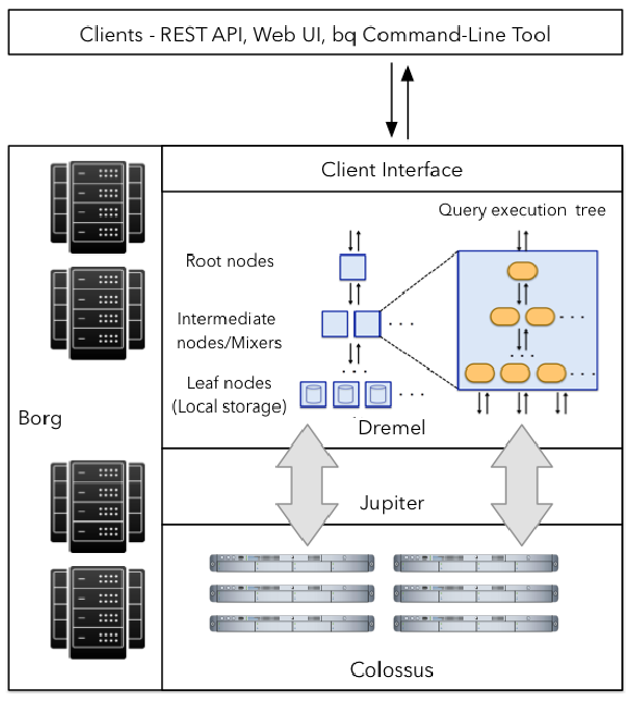
BigQuery traces its roots back to 2010, when Google released beta access to a new SQL processing system based on its distributed query engine technology, called Dremel, which was described in an influential paper released the same year. BigQuery and Dremel share the same underlying architecture and by incorporating columnar storage and tree architecture of Dremel, BigQuery manages to offer unprecedented performance. But, BigQuery is much more than Dremel which serves as the execution engine for the BigQuery. In fact, BigQuery service leverages Google’s innovative technologies like Borg – large-scale cluster management system, Colossus – Google’s latest generation distributed file system, Capacitor – columnar data storage format, and Jupiter – Google’s networking infrastructure. As illustrated below, a BigQuery client interact with Dremel engine via a client interface. Borg – Google’s large-scale cluster management system – allocates the compute capacity for the Dremel jobs. Dremel jobs read data from Google’s Colossus file systems using Jupiter network, perform various SQL operations and return results to the client.
Having previously worked with a number of other vendors which have successfully occupied this realm for a very long time, it was refreshing to see how different BigQuery is and what separates it from the rest of the competition. But before I get into the general observations and the actual conclusion, let’s look at how one can easily process, load and query large volumes of data (TPC-DS data in this example) using BigQuery and a few Python scripts for automation.
TPC-DS Schema Creation and Data Loading
BigQuery offers a number of ways one can interact with it and take advantage of its functionality. The most basic one is through the GCP Web UI but for repetitive tasks users will find themselves mainly utilising Google Cloud SDK or via Google BigQuery API. For the purpose of this example, I have generated two TPC-DS datasets – 100GB and 300GB – and staged them on the local machine’s folder. I have also created a TPC-DS schema JSON file which is used by the script to generate all dataset objects. All these resources, as well as the scripts used in this post can be found in my OneDrive folder HERE.
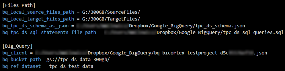
The following config file parameters and Python code are used to mainly clean up the flat files (TPC-DS delimits line ending with a “|” character which needs to be removed), break them up into smaller chunks and upload them to Google Cloud storage service (it assumes that gs://tpc_ds_data_100GB and gs://tpc_ds_data_300GB buckets has already been created). The schema structure used for this project is a direct translation of the PostgreSQL-specific TPC-DS schema used in one of my earlier projects where data types and their NULL-ability have been converted and standardized to conform to BigQuery standards.
import configparser
from tqdm import tqdm
from os import path, rename, listdir, remove, walk
from shutil import copy2, move
from google.cloud import storage
from csv import reader, writer


config = configparser.ConfigParser()
config.read("params.cfg")

bq_tpc_ds_schema_as_json = config.get(
    "Files_Path", path.normpath("bq_tpc_ds_schema_as_json"))
bq_local_source_files_path = config.get(
    "Files_Path", path.normpath("bq_local_source_files_path"))
bq_local_target_files_path = config.get(
    "Files_Path", path.normpath("bq_local_target_files_path"))
storage_client = config.get("Big_Query", path.normpath("bq_client"))
bq_bucket_path = config.get("Big_Query", "bq_bucket_path")
bq_storage_client = storage.Client.from_service_account_json(storage_client)


keep_src_files = True
keep_headers = False
keep_src_csv_files = True
row_limit = 1000000
output_name_template = '_%s.csv'
delimiter = '|'


def RemoveFiles(DirPath):
    filelist = [f for f in listdir(DirPath)]
    for f in filelist:
        remove(path.join(DirPath, f))


def SourceFilesRename(bq_local_source_files_path):
    for file in listdir(bq_local_source_files_path):
        if file.endswith(".dat"):
            rename(path.join(bq_local_source_files_path, file),
                   path.join(bq_local_source_files_path, file[:-4]+'.csv'))


def SplitLargeFiles(file, row_count, bq_local_target_files_path, output_name_template, keep_headers=False):
    """
    Split flat files into smaller chunks based on the comparison between row count
    and 'row_limit' variable value. This creates file_row_count/row_limit number of files which can
    facilitate upload speed if parallelized.
    """
    file_handler = open(path.join(bq_local_target_files_path, file), 'r')
    csv_reader = reader(file_handler, delimiter=delimiter)
    current_piece = 1
    current_out_path = path.join(bq_local_target_files_path, path.splitext(file)[
                                 0]+output_name_template % current_piece)
    current_out_writer = writer(
        open(current_out_path, 'w', newline=''), delimiter=delimiter)
    current_limit = row_limit
    if keep_headers:
        headers = next(csv_reader)
        current_out_writer.writerow(headers)
    pbar = tqdm(total=row_count)
    for i, row in enumerate(csv_reader):
        pbar.update()
        if i + 1 > current_limit:
            current_piece += 1
            current_limit = row_limit * current_piece
            current_out_path = path.join(bq_local_target_files_path, path.splitext(file)[
                                         0]+output_name_template % current_piece)
            current_out_writer = writer(
                open(current_out_path, 'w', newline=''), delimiter=delimiter)
            if keep_headers:
                current_out_writer.writerow(headers)
        current_out_writer.writerow(row)
    pbar.close()
    print("\n")


def ProcessLargeFiles(bq_local_source_files_path, bq_local_target_files_path, output_name_template, row_limit):
    """
    Remove trailing '|' characters from the files generated by the TPC-DS utility
    as they intefere with BQ load function. As BQ does not allow for denoting end-of-line
    characters in the flat file, this breaks data load functionality. This function also calls
    the 'SplitLargeFiles' function resulting in splitting files with the row count > 'row_limit'
    variable value into smaller chunks/files.
    """
    RemoveFiles(bq_local_target_files_path)
    fileRowCounts = []
    for file in listdir(bq_local_source_files_path):
        if file.endswith(".csv"):
            fileRowCounts.append([file, sum(1 for line in open(
                path.join(bq_local_source_files_path, file), newline=''))])
    for file in fileRowCounts:
        if file[1] > row_limit:
            print(
                "Removing trailing characters in {f} file...".format(f=file[0]))
            RemoveTrailingChar(row_limit, path.join(
                bq_local_source_files_path, file[0]), path.join(bq_local_target_files_path, file[0]))
            print("\nSplitting file:", file[0],)
            print("Measured row count:", file[1])
            print("Progress...")
            SplitLargeFiles(
                file[0], file[1], bq_local_target_files_path, output_name_template)
            remove(path.join(bq_local_target_files_path, file[0]))
        else:
            print(
                "Removing trailing characters in {f} file...".format(f=file[0]))
            RemoveTrailingChar(row_limit, path.join(
                bq_local_source_files_path, file[0]), path.join(bq_local_target_files_path, file[0]))
    RemoveFiles(bq_local_source_files_path)


def RemoveTrailingChar(row_limit, bq_local_source_files_path, bq_local_target_files_path):
    """
    Remove trailing '|' characters from files' line ending.
    """
    line_numer = row_limit
    lines = []
    with open(bq_local_source_files_path, "r") as r, open(bq_local_target_files_path, "w") as w:
        for line in r:
            if line.endswith('|\n'):
                lines.append(line[:-2]+"\n")
                if len(lines) == line_numer:
                    w.writelines(lines)
                    lines = []
        w.writelines(lines)


def GcsUploadBlob(bq_storage_client, bq_local_target_files_path, bq_bucket_path):
    """
    Upload files into the nominated GCP bucket if it does not exists.
    """
    bucket_name = (bq_bucket_path.split("//"))[1].split("/")[0]
    CHUNK_SIZE = 10485760
    bucket = bq_storage_client.get_bucket(bucket_name)
    print("\nCommencing files upload...")
    for file in listdir(bq_local_target_files_path):
        try:
            blob = bucket.blob(file, chunk_size=CHUNK_SIZE)
            file_exist = storage.Blob(bucket=bucket, name=file).exists(
                bq_storage_client)
            if not file_exist:
                print("Uploading file {fname} into {bname} GCP bucket...".format(
                    fname=file, bname=bucket_name))
                blob.upload_from_filename(
                    path.join(bq_local_target_files_path, file))
            else:
                print("Nominated file {fname} already exists in {bname} bucket. Moving on...".format(
                    fname=file, bname=bucket_name))
        except Exception as e:
            print(e)


if __name__ == "__main__":
    SourceFilesRename(bq_local_source_files_path)
    ProcessLargeFiles(bq_local_source_files_path,
                      bq_local_target_files_path, output_name_template, row_limit)
    GcsUploadBlob(bq_storage_client,
                  bq_local_target_files_path, bq_bucket_path)
Once all the TPC-DS data has been moved across into GCP storage bucket, we can proceed with creating BigQuery dataset (synonymous with the schema name in a typical Microsoft SQL Server or PostgreSQL RDBMS hierarchy) and its corresponding tables. Dataset is associated with a project which forms the overarching container, somewhat equivalent to the database if you come from a traditional RDBMS experience. It is also worth pointing out that dataset names must be unique per project, all tables referenced in a query must be stored in datasets in the same location and finally, geographic location can be set at creation time only. The following is an excerpt from the JSON file used to create the dataset schema which can be downloaded from my OneDrive folder HERE.
Now that the dataset is in place, we can create the required tables and populate them with the flat files data which was moved across into Google cloud storage using the previous code snippet. The following Python script creates tpc_ds_test_data dataset, creates all tables based on the TPC-DS schema stored in the JSON file and finally populates them with text files data.
from google.cloud import bigquery
from google.cloud.exceptions import NotFound
from google.cloud import storage
from os import path
import configparser
import json
import re


config = configparser.ConfigParser()
config.read("params.cfg")

bq_tpc_ds_schema_as_json = config.get(
    "Files_Path", path.normpath("bq_tpc_ds_schema_as_json"))
bq_client = config.get("Big_Query", path.normpath("bq_client"))
bq_client = bigquery.Client.from_service_account_json(bq_client)
storage_client = config.get("Big_Query", path.normpath("bq_client"))
bq_bucket_path = config.get("Big_Query", "bq_bucket_path")
bq_storage_client = storage.Client.from_service_account_json(storage_client)
bq_ref_dataset = config.get("Big_Query", "bq_ref_dataset")


def dataset_bq_exists(bq_client, bq_ref_dataset):
    try:
        bq_client.get_dataset(bq_ref_dataset)
        return True
    except NotFound as e:
        return False


def bq_create_dataset(bq_client, bq_ref_dataset):
    """
    Create BigQuery dataset if it does not exists in the
    Australian location
    """
    if not dataset_bq_exists(bq_client, bq_ref_dataset):
        print("Creating {d} dataset...".format(d=bq_ref_dataset))
        dataset = bq_client.dataset(bq_ref_dataset)
        dataset = bigquery.Dataset(dataset)
        dataset.location = 'australia-southeast1'
        dataset = bq_client.create_dataset(dataset)
    else:
        print("Nominated dataset already exists. Moving on...")


def table_bq_exists(bq_client, ref_table):
    try:
        bq_client.get_table(ref_table)
        return True
    except NotFound as e:
        return False


def bq_drop_create_table(bq_client, bq_ref_dataset, bq_tpc_ds_schema_as_json):
    """
    Drop (if exists) and create schema tables on the nominated BigQuery dataset.
    Schema details are stored inside 'tpc_ds_schema.json' file.
    """
    dataset = bq_client.dataset(bq_ref_dataset)
    with open(bq_tpc_ds_schema_as_json) as schema_file:
        data = json.load(schema_file)
        for t in data['table_schema']:
            table_name = t['table_name']
            ref_table = dataset.table(t['table_name'])
            table = bigquery.Table(ref_table)
            if table_bq_exists(bq_client, ref_table):
                print("Table '{tname}' already exists in the '{dname}' dataset. Dropping table '{tname}'...".format(
                    tname=table_name, dname=bq_ref_dataset))
                bq_client.delete_table(table)
            for f in t['fields']:
                table.schema += (
                    bigquery.SchemaField(f['name'], f['type'], mode=f['mode']),)
            print("Creating table {tname} in the '{dname}' dataset...".format(
                tname=table_name, dname=bq_ref_dataset))
            table = bq_client.create_table(table)


def bq_load_data_from_file(bq_client, bq_ref_dataset,  bq_bucket_path, bq_storage_client):
    """
    Load data stored on the nominated GCP bucket into dataset tables
    """
    bucket_name = (bq_bucket_path.split("//"))[1].split("/")[0]
    bucket = bq_storage_client.get_bucket(bucket_name)
    blobs = bucket.list_blobs()
    dataset = bq_client.dataset(bq_ref_dataset)
    for blob in blobs:
        file_name = blob.name
        rem_char = re.findall("_\d+", file_name)
        if len(rem_char) == 0:
            ref_table = dataset.table(file_name[:file_name.index(".")])
            table_name = file_name[:file_name.index(".")]
        else:
            rem_char = str("".join(rem_char))
            ref_table = dataset.table(file_name[:file_name.index(rem_char)])
            table_name = file_name[:file_name.index(rem_char)]
        print("Loading file {f} into {t} table...".format(
            f=file_name, t=table_name))
        job_config = bigquery.LoadJobConfig()
        job_config.source_format = "CSV"
        job_config.skip_leading_rows = 0
        job_config.field_delimiter = "|"
        job_config.write_disposition = bigquery.WriteDisposition.WRITE_APPEND
        job = bq_client.load_table_from_uri(
            path.join(bq_bucket_path, file_name), ref_table, job_config=job_config)
        result = job.result()
        print(result.state)


if __name__ == "__main__":
    bq_create_dataset(bq_client, bq_ref_dataset)
    bq_drop_create_table(bq_client, bq_ref_dataset, bq_tpc_ds_schema_as_json)
    bq_load_data_from_file(bq_client, bq_ref_dataset,
                           bq_bucket_path, bq_storage_client)
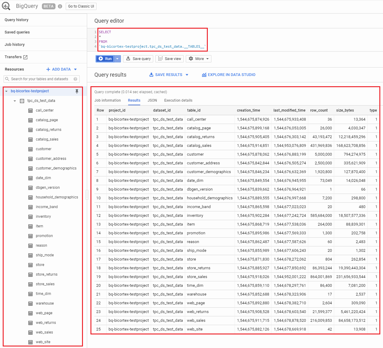
BigQuery offers some special tables whose contents represent metadata, such as the list of tables and views in a dataset. To confirm all objects have been created in the correct dataset, we can interrogate the __TABLES__ or __TABLES_SUMMARY__ meta-tables as per the query below.
In the next post I will go over some of TPC-DS queries execution performance on BigQuery, BigQuery ML – Google’s take on in-database machine learning as well as some basic interactive dashboard building in Tableau.
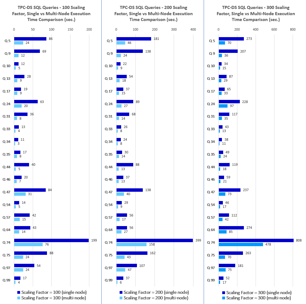
In the previous post I started looking at some of the TPC-DS queries’ performance across a single node and multi-node environments. This post continues with the theme of performance analysis across the remaining set of queries and looks at high-level interactions between Vertica and Tableau/PowerBI. Firstly though, let’s look at the remaining ten queries and how their execution times fared in the context of three different data and cluster sizes.
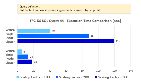
--Query 44
SELECT asceding.rnk,
               i1.i_product_name best_performing,
               i2.i_product_name worst_performing
FROM  (SELECT *
       FROM   (SELECT item_sk,
                      Rank()
                        OVER (
                          ORDER BY rank_col ASC) rnk
               FROM   (SELECT ss_item_sk         item_sk,
                              Avg(ss_net_profit) rank_col
                       FROM   tpc_ds.store_sales ss1
                       WHERE  ss_store_sk = 4
                       GROUP  BY ss_item_sk
                       HAVING Avg(ss_net_profit) > 0.9 *
                              (SELECT Avg(ss_net_profit)
                                      rank_col
                               FROM   tpc_ds.store_sales
                               WHERE  ss_store_sk = 4
                                      AND ss_cdemo_sk IS
                                          NULL
                               GROUP  BY ss_store_sk))V1)
              V11
       WHERE  rnk < 11) asceding,
      (SELECT *
       FROM   (SELECT item_sk,
                      Rank()
                        OVER (
                          ORDER BY rank_col DESC) rnk
               FROM   (SELECT ss_item_sk         item_sk,
                              Avg(ss_net_profit) rank_col
                       FROM   tpc_ds.store_sales ss1
                       WHERE  ss_store_sk = 4
                       GROUP  BY ss_item_sk
                       HAVING Avg(ss_net_profit) > 0.9 *
                              (SELECT Avg(ss_net_profit)
                                      rank_col
                               FROM   tpc_ds.store_sales
                               WHERE  ss_store_sk = 4
                                      AND ss_cdemo_sk IS
                                          NULL
                               GROUP  BY ss_store_sk))V2)
              V21
       WHERE  rnk < 11) descending,
      tpc_ds.item i1,
      tpc_ds.item i2
WHERE  asceding.rnk = descending.rnk
       AND i1.i_item_sk = asceding.item_sk
       AND i2.i_item_sk = descending.item_sk
ORDER  BY asceding.rnk
LIMIT 100;
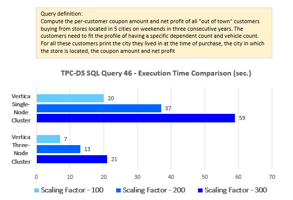
--Query 46
SELECT c_last_name,
               c_first_name,
               ca_city,
               bought_city,
               ss_ticket_number,
               amt,
               profit
FROM   (SELECT ss_ticket_number,
               ss_customer_sk,
               ca_city            bought_city,
               Sum(ss_coupon_amt) amt,
               Sum(ss_net_profit) profit
        FROM   tpc_ds.store_sales,
               tpc_ds.date_dim,
               tpc_ds.store,
               tpc_ds.household_demographics,
               tpc_ds.customer_address
        WHERE  store_sales.ss_sold_date_sk = date_dim.d_date_sk
               AND store_sales.ss_store_sk = store.s_store_sk
               AND store_sales.ss_hdemo_sk = household_demographics.hd_demo_sk
               AND store_sales.ss_addr_sk = customer_address.ca_address_sk
               AND ( household_demographics.hd_dep_count = 6
                      OR household_demographics.hd_vehicle_count = 0 )
               AND date_dim.d_dow IN ( 6, 0 )
               AND date_dim.d_year IN ( 2000, 2000 + 1, 2000 + 2 )
               AND store.s_city IN ( 'Midway', 'Fairview', 'Fairview',
                                     'Fairview',
                                     'Fairview' )
        GROUP  BY ss_ticket_number,
                  ss_customer_sk,
                  ss_addr_sk,
                  ca_city) dn,
       tpc_ds.customer,
       tpc_ds.customer_address current_addr
WHERE  ss_customer_sk = c_customer_sk
       AND customer.c_current_addr_sk = current_addr.ca_address_sk
       AND current_addr.ca_city <> bought_city
ORDER  BY c_last_name,
          c_first_name,
          ca_city,
          bought_city,
          ss_ticket_number
LIMIT 100;
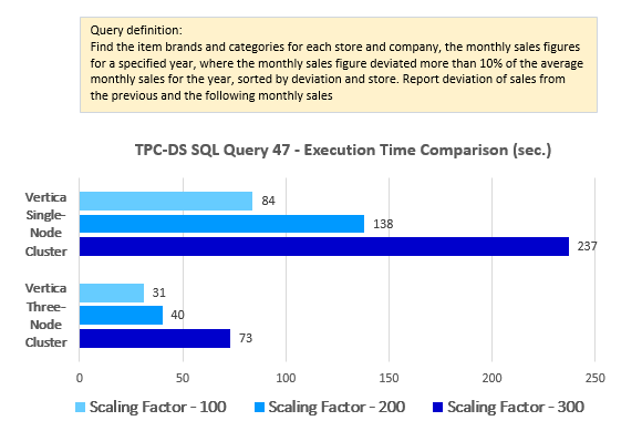
--Query 47
WITH v1
     AS (SELECT i_category,
                i_brand,
                s_store_name,
                s_company_name,
                d_year,
                d_moy,
                Sum(ss_sales_price)         sum_sales,
                Avg(Sum(ss_sales_price))
                  OVER (
                    partition BY i_category, i_brand, s_store_name,
                  s_company_name,
                  d_year)
                                            avg_monthly_sales,
                Rank()
                  OVER (
                    partition BY i_category, i_brand, s_store_name,
                  s_company_name
                    ORDER BY d_year, d_moy) rn
         FROM   tpc_ds.item,
                tpc_ds.store_sales,
                tpc_ds.date_dim,
                tpc_ds.store
         WHERE  ss_item_sk = i_item_sk
                AND ss_sold_date_sk = d_date_sk
                AND ss_store_sk = s_store_sk
                AND ( d_year = 1999
                       OR ( d_year = 1999 - 1
                            AND d_moy = 12 )
                       OR ( d_year = 1999 + 1
                            AND d_moy = 1 ) )
         GROUP  BY i_category,
                   i_brand,
                   s_store_name,
                   s_company_name,
                   d_year,
                   d_moy),
     v2
     AS (SELECT v1.i_category,
                v1.d_year,
                v1.d_moy,
                v1.avg_monthly_sales,
                v1.sum_sales,
                v1_lag.sum_sales  psum,
                v1_lead.sum_sales nsum
         FROM   v1,
                v1 v1_lag,
                v1 v1_lead
         WHERE  v1.i_category = v1_lag.i_category
                AND v1.i_category = v1_lead.i_category
                AND v1.i_brand = v1_lag.i_brand
                AND v1.i_brand = v1_lead.i_brand
                AND v1.s_store_name = v1_lag.s_store_name
                AND v1.s_store_name = v1_lead.s_store_name
                AND v1.s_company_name = v1_lag.s_company_name
                AND v1.s_company_name = v1_lead.s_company_name
                AND v1.rn = v1_lag.rn + 1
                AND v1.rn = v1_lead.rn - 1)
SELECT *
FROM   v2
WHERE  d_year = 1999
       AND avg_monthly_sales > 0
       AND CASE
             WHEN avg_monthly_sales > 0 THEN Abs(sum_sales - avg_monthly_sales)
                                             /
                                             avg_monthly_sales
             ELSE NULL
           END > 0.1
ORDER  BY sum_sales - avg_monthly_sales,
          3
LIMIT 100;
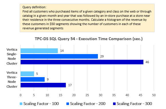
--Query 54
WITH my_customers
     AS (SELECT DISTINCT c_customer_sk,
                         c_current_addr_sk
         FROM   (SELECT cs_sold_date_sk     sold_date_sk,
                        cs_bill_customer_sk customer_sk,
                        cs_item_sk          item_sk
                 FROM   tpc_ds.catalog_sales
                 UNION ALL
                 SELECT ws_sold_date_sk     sold_date_sk,
                        ws_bill_customer_sk customer_sk,
                        ws_item_sk          item_sk
                 FROM   tpc_ds.web_sales) cs_or_ws_sales,
                tpc_ds.item,
                tpc_ds.date_dim,
                tpc_ds.customer
         WHERE  sold_date_sk = d_date_sk
                AND item_sk = i_item_sk
                AND i_category = 'Sports'
                AND i_class = 'fitness'
                AND c_customer_sk = cs_or_ws_sales.customer_sk
                AND d_moy = 5
                AND d_year = 2000),
     my_revenue
     AS (SELECT c_customer_sk,
                Sum(ss_ext_sales_price) AS revenue
         FROM   my_customers,
                tpc_ds.store_sales,
                tpc_ds.customer_address,
                tpc_ds.store,
                tpc_ds.date_dim
         WHERE  c_current_addr_sk = ca_address_sk
                AND ca_county = s_county
                AND ca_state = s_state
                AND ss_sold_date_sk = d_date_sk
                AND c_customer_sk = ss_customer_sk
                AND d_month_seq BETWEEN (SELECT DISTINCT d_month_seq + 1
                                         FROM   tpc_ds.date_dim
                                         WHERE  d_year = 2000
                                                AND d_moy = 5) AND
                                        (SELECT DISTINCT
                                        d_month_seq + 3
                                         FROM   tpc_ds.date_dim
                                         WHERE  d_year = 2000
                                                AND d_moy = 5)
         GROUP  BY c_customer_sk),
     segments
     AS (SELECT Cast(( revenue / 50 ) AS INT) AS segment
         FROM   my_revenue)
SELECT segment,
               Count(*)     AS num_customers,
               segment * 50 AS segment_base
FROM   segments
GROUP  BY segment
ORDER  BY segment,
          num_customers
LIMIT 100;
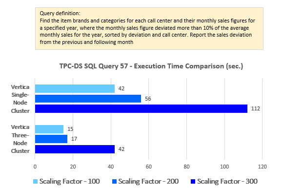
--Query 57
WITH v1
     AS (SELECT i_category,
                i_brand,
                cc_name,
                d_year,
                d_moy,
                Sum(cs_sales_price)                                    sum_sales
                ,
                Avg(Sum(cs_sales_price))
                  OVER (
                    partition BY i_category, i_brand, cc_name, d_year)
                avg_monthly_sales
                   ,
                Rank()
                  OVER (
                    partition BY i_category, i_brand, cc_name
                    ORDER BY d_year, d_moy)                            rn
         FROM   tpc_ds.item,
                tpc_ds.catalog_sales,
                tpc_ds.date_dim,
                tpc_ds.call_center
         WHERE  cs_item_sk = i_item_sk
                AND cs_sold_date_sk = d_date_sk
                AND cc_call_center_sk = cs_call_center_sk
                AND ( d_year = 2000
                       OR ( d_year = 2000 - 1
                            AND d_moy = 12 )
                       OR ( d_year = 2000 + 1
                            AND d_moy = 1 ) )
         GROUP  BY i_category,
                   i_brand,
                   cc_name,
                   d_year,
                   d_moy),
     v2
     AS (SELECT v1.i_brand,
                v1.d_year,
                v1.avg_monthly_sales,
                v1.sum_sales,
                v1_lag.sum_sales  psum,
                v1_lead.sum_sales nsum
         FROM   v1,
                v1 v1_lag,
                v1 v1_lead
         WHERE  v1.i_category = v1_lag.i_category
                AND v1.i_category = v1_lead.i_category
                AND v1.i_brand = v1_lag.i_brand
                AND v1.i_brand = v1_lead.i_brand
                AND v1. cc_name = v1_lag. cc_name
                AND v1. cc_name = v1_lead. cc_name
                AND v1.rn = v1_lag.rn + 1
                AND v1.rn = v1_lead.rn - 1)
SELECT *
FROM   v2
WHERE  d_year = 2000
       AND avg_monthly_sales > 0
       AND CASE
             WHEN avg_monthly_sales > 0 THEN Abs(sum_sales - avg_monthly_sales)
                                             /
                                             avg_monthly_sales
             ELSE NULL
           END > 0.1
ORDER  BY sum_sales - avg_monthly_sales,
          3
LIMIT 100;
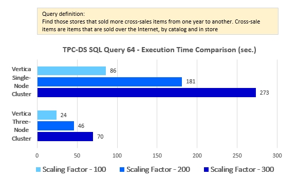
--Query 64
WITH cs_ui
     AS (SELECT cs_item_sk,
                Sum(cs_ext_list_price) AS sale,
                Sum(cr_refunded_cash + cr_reversed_charge
                    + cr_store_credit) AS refund
         FROM   tpc_ds.catalog_sales,
                tpc_ds.catalog_returns
         WHERE  cs_item_sk = cr_item_sk
                AND cs_order_number = cr_order_number
         GROUP  BY cs_item_sk
         HAVING Sum(cs_ext_list_price) > 2 * Sum(
                cr_refunded_cash + cr_reversed_charge
                + cr_store_credit)),
     cross_sales
     AS (SELECT i_product_name         product_name,
                i_item_sk              item_sk,
                s_store_name           store_name,
                s_zip                  store_zip,
                ad1.ca_street_number   b_street_number,
                ad1.ca_street_name     b_streen_name,
                ad1.ca_city            b_city,
                ad1.ca_zip             b_zip,
                ad2.ca_street_number   c_street_number,
                ad2.ca_street_name     c_street_name,
                ad2.ca_city            c_city,
                ad2.ca_zip             c_zip,
                d1.d_year              AS syear,
                d2.d_year              AS fsyear,
                d3.d_year              s2year,
                Count(*)               cnt,
                Sum(ss_wholesale_cost) s1,
                Sum(ss_list_price)     s2,
                Sum(ss_coupon_amt)     s3
         FROM   tpc_ds.store_sales,
                tpc_ds.store_returns,
                cs_ui,
                tpc_ds.date_dim d1,
                tpc_ds.date_dim d2,
                tpc_ds.date_dim d3,
                tpc_ds.store,
                tpc_ds.customer,
                tpc_ds.customer_demographics cd1,
                tpc_ds.customer_demographics cd2,
                tpc_ds.promotion,
                tpc_ds.household_demographics hd1,
                tpc_ds.household_demographics hd2,
                tpc_ds.customer_address ad1,
                tpc_ds.customer_address ad2,
                tpc_ds.income_band ib1,
                tpc_ds.income_band ib2,
                tpc_ds.item
         WHERE  ss_store_sk = s_store_sk
                AND ss_sold_date_sk = d1.d_date_sk
                AND ss_customer_sk = c_customer_sk
                AND ss_cdemo_sk = cd1.cd_demo_sk
                AND ss_hdemo_sk = hd1.hd_demo_sk
                AND ss_addr_sk = ad1.ca_address_sk
                AND ss_item_sk = i_item_sk
                AND ss_item_sk = sr_item_sk
                AND ss_ticket_number = sr_ticket_number
                AND ss_item_sk = cs_ui.cs_item_sk
                AND c_current_cdemo_sk = cd2.cd_demo_sk
                AND c_current_hdemo_sk = hd2.hd_demo_sk
                AND c_current_addr_sk = ad2.ca_address_sk
                AND c_first_sales_date_sk = d2.d_date_sk
                AND c_first_shipto_date_sk = d3.d_date_sk
                AND ss_promo_sk = p_promo_sk
                AND hd1.hd_income_band_sk = ib1.ib_income_band_sk
                AND hd2.hd_income_band_sk = ib2.ib_income_band_sk
                AND cd1.cd_marital_status <> cd2.cd_marital_status
                AND i_color IN ( 'cyan', 'peach', 'blush', 'frosted',
                                 'powder', 'orange' )
                AND i_current_price BETWEEN 58 AND 58 + 10
                AND i_current_price BETWEEN 58 + 1 AND 58 + 15
         GROUP  BY i_product_name,
                   i_item_sk,
                   s_store_name,
                   s_zip,
                   ad1.ca_street_number,
                   ad1.ca_street_name,
                   ad1.ca_city,
                   ad1.ca_zip,
                   ad2.ca_street_number,
                   ad2.ca_street_name,
                   ad2.ca_city,
                   ad2.ca_zip,
                   d1.d_year,
                   d2.d_year,
                   d3.d_year)
SELECT cs1.product_name,
       cs1.store_name,
       cs1.store_zip,
       cs1.b_street_number,
       cs1.b_streen_name,
       cs1.b_city,
       cs1.b_zip,
       cs1.c_street_number,
       cs1.c_street_name,
       cs1.c_city,
       cs1.c_zip,
       cs1.syear,
       cs1.cnt,
       cs1.s1,
       cs1.s2,
       cs1.s3,
       cs2.s1,
       cs2.s2,
       cs2.s3,
       cs2.syear,
       cs2.cnt
FROM   cross_sales cs1,
       cross_sales cs2
WHERE  cs1.item_sk = cs2.item_sk
       AND cs1.syear = 2001
       AND cs2.syear = 2001 + 1
       AND cs2.cnt <= cs1.cnt
       AND cs1.store_name = cs2.store_name
       AND cs1.store_zip = cs2.store_zip
ORDER  BY cs1.product_name,
          cs1.store_name,
          cs2.cnt;
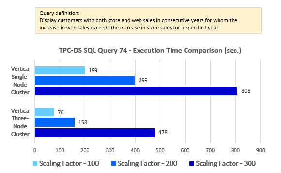
--Query 74
WITH year_total
     AS (SELECT c_customer_id    customer_id,
                c_first_name     customer_first_name,
                c_last_name      customer_last_name,
                d_year           AS year1,
                Sum(ss_net_paid) year_total,
                's'              sale_type
         FROM   tpc_ds.customer,
                tpc_ds.store_sales,
                tpc_ds.date_dim
         WHERE  c_customer_sk = ss_customer_sk
                AND ss_sold_date_sk = d_date_sk
                AND d_year IN ( 1999, 1999 + 1 )
         GROUP  BY c_customer_id,
                   c_first_name,
                   c_last_name,
                   d_year
         UNION ALL
         SELECT c_customer_id    customer_id,
                c_first_name     customer_first_name,
                c_last_name      customer_last_name,
                d_year           AS year1,
                Sum(ws_net_paid) year_total,
                'w'              sale_type
         FROM   tpc_ds.customer,
                tpc_ds.web_sales,
                tpc_ds.date_dim
         WHERE  c_customer_sk = ws_bill_customer_sk
                AND ws_sold_date_sk = d_date_sk
                AND d_year IN ( 1999, 1999 + 1 )
         GROUP  BY c_customer_id,
                   c_first_name,
                   c_last_name,
                   d_year)
SELECT t_s_secyear.customer_id,
               t_s_secyear.customer_first_name,
               t_s_secyear.customer_last_name
FROM   year_total t_s_firstyear,
       year_total t_s_secyear,
       year_total t_w_firstyear,
       year_total t_w_secyear
WHERE  t_s_secyear.customer_id = t_s_firstyear.customer_id
       AND t_s_firstyear.customer_id = t_w_secyear.customer_id
       AND t_s_firstyear.customer_id = t_w_firstyear.customer_id
       AND t_s_firstyear.sale_type = 's'
       AND t_w_firstyear.sale_type = 'w'
       AND t_s_secyear.sale_type = 's'
       AND t_w_secyear.sale_type = 'w'
       AND t_s_firstyear.year1 = 1999
       AND t_s_secyear.year1 = 1999 + 1
       AND t_w_firstyear.year1 = 1999
       AND t_w_secyear.year1 = 1999 + 1
       AND t_s_firstyear.year_total > 0
       AND t_w_firstyear.year_total > 0
       AND CASE
             WHEN t_w_firstyear.year_total > 0 THEN t_w_secyear.year_total /
                                                    t_w_firstyear.year_total
             ELSE NULL
           END > CASE
                   WHEN t_s_firstyear.year_total > 0 THEN
                   t_s_secyear.year_total /
                   t_s_firstyear.year_total
                   ELSE NULL
                 END
ORDER  BY 1,
          2,
          3
LIMIT 100;
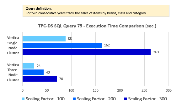
--Query 75
WITH all_sales
     AS (SELECT d_year,
                i_brand_id,
                i_class_id,
                i_category_id,
                i_manufact_id,
                Sum(sales_cnt) AS sales_cnt,
                Sum(sales_amt) AS sales_amt
         FROM   (SELECT d_year,
                        i_brand_id,
                        i_class_id,
                        i_category_id,
                        i_manufact_id,
                        cs_quantity - COALESCE(cr_return_quantity, 0)        AS
                        sales_cnt,
                        cs_ext_sales_price - COALESCE(cr_return_amount, 0.0) AS
                        sales_amt
                 FROM   tpc_ds.catalog_sales
                        JOIN tpc_ds.item
                          ON i_item_sk = cs_item_sk
                        JOIN tpc_ds.date_dim
                          ON d_date_sk = cs_sold_date_sk
                        LEFT JOIN tpc_ds.catalog_returns
                               ON ( cs_order_number = cr_order_number
                                    AND cs_item_sk = cr_item_sk )
                 WHERE  i_category = 'Men'
                 UNION
                 SELECT d_year,
                        i_brand_id,
                        i_class_id,
                        i_category_id,
                        i_manufact_id,
                        ss_quantity - COALESCE(sr_return_quantity, 0)     AS
                        sales_cnt,
                        ss_ext_sales_price - COALESCE(sr_return_amt, 0.0) AS
                        sales_amt
                 FROM   tpc_ds.store_sales
                        JOIN tpc_ds.item
                          ON i_item_sk = ss_item_sk
                        JOIN tpc_ds.date_dim
                          ON d_date_sk = ss_sold_date_sk
                        LEFT JOIN tpc_ds.store_returns
                               ON ( ss_ticket_number = sr_ticket_number
                                    AND ss_item_sk = sr_item_sk )
                 WHERE  i_category = 'Men'
                 UNION
                 SELECT d_year,
                        i_brand_id,
                        i_class_id,
                        i_category_id,
                        i_manufact_id,
                        ws_quantity - COALESCE(wr_return_quantity, 0)     AS
                        sales_cnt,
                        ws_ext_sales_price - COALESCE(wr_return_amt, 0.0) AS
                        sales_amt
                 FROM   tpc_ds.web_sales
                        JOIN tpc_ds.item
                          ON i_item_sk = ws_item_sk
                        JOIN tpc_ds.date_dim
                          ON d_date_sk = ws_sold_date_sk
                        LEFT JOIN tpc_ds.web_returns
                               ON ( ws_order_number = wr_order_number
                                    AND ws_item_sk = wr_item_sk )
                 WHERE  i_category = 'Men') sales_detail
         GROUP  BY d_year,
                   i_brand_id,
                   i_class_id,
                   i_category_id,
                   i_manufact_id)
SELECT prev_yr.d_year                        AS prev_year,
               curr_yr.d_year                        AS year1,
               curr_yr.i_brand_id,
               curr_yr.i_class_id,
               curr_yr.i_category_id,
               curr_yr.i_manufact_id,
               prev_yr.sales_cnt                     AS prev_yr_cnt,
               curr_yr.sales_cnt                     AS curr_yr_cnt,
               curr_yr.sales_cnt - prev_yr.sales_cnt AS sales_cnt_diff,
               curr_yr.sales_amt - prev_yr.sales_amt AS sales_amt_diff
FROM   all_sales curr_yr,
       all_sales prev_yr
WHERE  curr_yr.i_brand_id = prev_yr.i_brand_id
       AND curr_yr.i_class_id = prev_yr.i_class_id
       AND curr_yr.i_category_id = prev_yr.i_category_id
       AND curr_yr.i_manufact_id = prev_yr.i_manufact_id
       AND curr_yr.d_year = 2002
       AND prev_yr.d_year = 2002 - 1
       AND Cast(curr_yr.sales_cnt AS DECIMAL(17, 2)) / Cast(prev_yr.sales_cnt AS
                                                                DECIMAL(17, 2))
           < 0.9
ORDER  BY sales_cnt_diff
LIMIT 100;
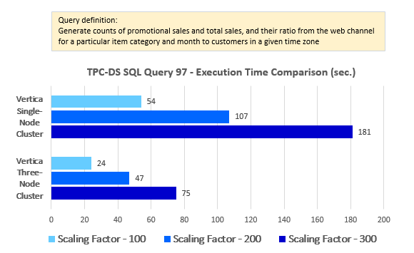
--Query 97
WITH ssci
     AS (SELECT ss_customer_sk customer_sk,
                ss_item_sk     item_sk
         FROM   tpc_ds.store_sales,
                tpc_ds.date_dim
         WHERE  ss_sold_date_sk = d_date_sk
                AND d_month_seq BETWEEN 1196 AND 1196 + 11
         GROUP  BY ss_customer_sk,
                   ss_item_sk),
     csci
     AS (SELECT cs_bill_customer_sk customer_sk,
                cs_item_sk          item_sk
         FROM   tpc_ds.catalog_sales,
                tpc_ds.date_dim
         WHERE  cs_sold_date_sk = d_date_sk
                AND d_month_seq BETWEEN 1196 AND 1196 + 11
         GROUP  BY cs_bill_customer_sk,
                   cs_item_sk)
SELECT Sum(CASE
                     WHEN ssci.customer_sk IS NOT NULL
                          AND csci.customer_sk IS NULL THEN 1
                     ELSE 0
                   END) store_only,
               Sum(CASE
                     WHEN ssci.customer_sk IS NULL
                          AND csci.customer_sk IS NOT NULL THEN 1
                     ELSE 0
                   END) catalog_only,
               Sum(CASE
                     WHEN ssci.customer_sk IS NOT NULL
                          AND csci.customer_sk IS NOT NULL THEN 1
                     ELSE 0
                   END) store_and_catalog
FROM   ssci
       FULL OUTER JOIN csci
                    ON ( ssci.customer_sk = csci.customer_sk
                         AND ssci.item_sk = csci.item_sk )
LIMIT 100;
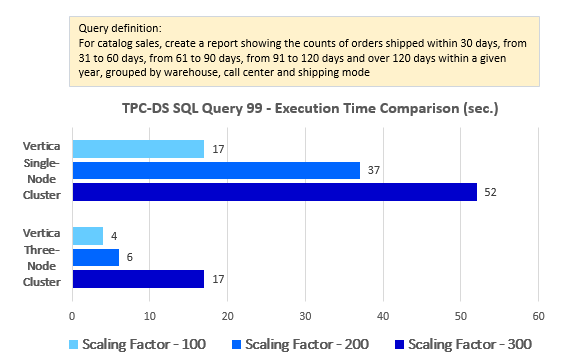
--Query 99
SELECT Substr(w_warehouse_name, 1, 20),
               sm_type,
               cc_name,
               Sum(CASE
                     WHEN ( cs_ship_date_sk - cs_sold_date_sk <= 30 ) THEN 1
                     ELSE 0
                   END) AS '30 days',
               Sum(CASE
                     WHEN ( cs_ship_date_sk - cs_sold_date_sk > 30 )
                          AND ( cs_ship_date_sk - cs_sold_date_sk <= 60 ) THEN 1
                     ELSE 0
                   END) AS '31-60 days',
               Sum(CASE
                     WHEN ( cs_ship_date_sk - cs_sold_date_sk > 60 )
                          AND ( cs_ship_date_sk - cs_sold_date_sk <= 90 ) THEN 1
                     ELSE 0
                   END) AS '61-90 days',
               Sum(CASE
                     WHEN ( cs_ship_date_sk - cs_sold_date_sk > 90 )
                          AND ( cs_ship_date_sk - cs_sold_date_sk <= 120 ) THEN
                     1
                     ELSE 0
                   END) AS '91-120 days',
               Sum(CASE
                     WHEN ( cs_ship_date_sk - cs_sold_date_sk > 120 ) THEN 1
                     ELSE 0
                   END) AS '>120 days'
FROM   tpc_ds.catalog_sales,
       tpc_ds.warehouse,
       tpc_ds.ship_mode,
       tpc_ds.call_center,
       tpc_ds.date_dim
WHERE  d_month_seq BETWEEN 1200 AND 1200 + 11
       AND cs_ship_date_sk = d_date_sk
       AND cs_warehouse_sk = w_warehouse_sk
       AND cs_ship_mode_sk = sm_ship_mode_sk
       AND cs_call_center_sk = cc_call_center_sk
GROUP  BY Substr(w_warehouse_name, 1, 20),
          sm_type,
          cc_name
ORDER  BY Substr(w_warehouse_name, 1, 20),
          sm_type,
          cc_name
LIMIT 100;
I didn’t set out on this experiment to compare Vertica’s performance to other vendors in the MPP category, so I cannot comment on how it could verse against other RDBMS systems. It would have been interesting to see how, for example, Pivotal’s Greenplum would match up when testing it out on the identical hardware and data volumes but this 4-part series was primarily focused on establishing the connection between the two variables: the number of nodes and data size. From that perspective, Vertica performs very well ‘out-of-the-box’, and without any tuning or tweaking it managed to not only execute the queries relatively fast (given the mediocre hardware specs) but also take full advantage of the extra computing resources to distribute the load across the available nodes and cut queries execution times.
Looking at the results and how they present the dichotomies across the multitude of different configurations, the first thing that jumps out is the fact the differences between performance levels across various data volumes and node counts are very linear. On an average, the query execution speed doubles for every scaling factor increase and goes down by a factor of two for every node that’s removed. There are some slight variations but on the whole Vertica performance is consistent and predictable, and all twenty queries exhibiting similar pattern when dealing with more data and/or more computing power thrown at it (additional nodes).
Looking at the side-by-side comparison of the execution results across single and multi-node configurations the differences between across scaling factors of 100, 200 and 300 are very consistent (click on image to expand).
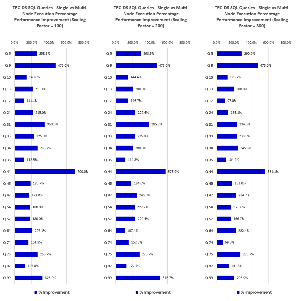
Converting these differences (single vs multi-node deployment) into percentage yielded an average of 243% increase for the scaling factor of 100, 252% increase for the scaling factor of 200 and 217% increase for the scaling factor of 300 as per the chart below (click on image to expand).
Finally, let’s look at how Vertica (three-node cluster with 100 scaling factor TPC-DS data) performed against some ad hoc generated queries in PowerBI and Tableau applications. Below are two short video clips depicting a rudimentary analysis of store sales data (this fact table contains close to 300 million records) against date, item, store and customer_address dimensions. It’s the type of rapid-fire, exploratory analysis one would conduct to analyse retail data to answer some immediate questions. I also set up Tableau and PowerBI side-by-side a process viewer/system monitor (htop), with four panes displaying core performance metrics e.g. CPU load, swap, memory status etc. across the three nodes and the machine hosting visualisation application (bottom view) so that I could observer (and record) systems’ behaviour when interactively aggregating data. In this way it was easy to see load distribution and how each host reacted (performance-wise) to queries issued based on this analysis. With respect to PowerBI, you can see that my three years old work laptop I recorded this on was not up to the task due to large amount of CPU cycles consumed by screen-recording software alone. On the flip side, Tableau run on my dual-CPU Mac Pro so the whole process was stutter-free and could reflect the fact that given access to a better hardware, PowerBI may also perform better.
I used Tableau Desktop version 2018.1 with native support for Vertica. As opposed to PowerBI, Tableau had no issues reading data from ‘customer’ dimension but in order to make those two footages as comparable as possible I abandoned it and used ‘customer_address’ instead. In terms of raw performance, this mini-cluster actually turned out to be borderline usable and in most cases I didn’t need to wait more than 10 seconds for aggregation or filtering to complete. Each node CPU spiked close to 100 percent during queries execution but given the volume of data and the mediocre hardware this data was crunched on, I would say that Vertica performed quite well.
PowerBI version 2.59 (used in the below footage) included Vertica support in Beta only so chances are the final release will be much better supported and optimised. PowerBI wasn’t too cooperative when selecting the data out of ‘customer’ dimension (see footage below) but everything else worked as expected e.g. geospatial analysis, various graphs etc. Performance-wise, I still think that Tableau was more workable but given the fact that Vertica support was still in preview and my pedestrian-quality laptop I was testing it on, chances are that PowerBI would be a viable choice for such exploratory analysis, especially when factoring in the price – free!
Conclusion
There isn’t much I can add to what I have already stated based on my observations and performance results. Vertica easy set-up and hassle-free, almost plug-in configuration has made it very easy to work with. While I haven’t covered most of its ‘knobs and switches’ that come built-it to fine-tune some of its functionality, the installation process was simple and more intuitive the some of the other commercial RDBMS products out there, even the ones which come with pre-built binaries and executable packages. I only wish Vertica come with the latest Ubuntu Server LTS version support as the time of writing this post Ubuntu Bionic Beaver was the latest LTS release while Vertica 9.1 Ubuntu support only extended to version 14, dating back to July 2016 and supported only until April 2019.
Performance-wise, Vertica exceeded my expectations. Running on hardware which I had no real use for and originally intended to sell on Ebay for a few hundred dollars (if lucky), it managed to crunch through large volumes of data (by relative standards) in a very respectable time. Some of the more processing-intensive queries executed in seconds and scaled well (linearly) across additional nodes and increased data volumes. It would be a treat to compare it against the likes of Greenplum or CitusDB and explore some of its other features e.g. Machine Learning or Hadoop integration (an idea for a future blog) as SQL queries execution speed on structured data isn’t its only forte.
My name is Martin and this site is a random collection of recipes and reflections about various topics covering information management, data engineering, machine learning, business intelligence and visualisation plus everything else that I fancy to categorise under the 'analytics' umbrella. I'm a native of Poland but since my university days I have lived in Melbourne, Australia and worked as a DBA, developer, data architect, technical lead and team manager. My main interests lie in both, helping clients in technical aspects of information management e.g. data modelling, systems architecture, cloud deployments as well as business-oriented strategies e.g. enterprise data solutions project management, data governance and stewardship, data security and privacy or data monetisation. On the whole, I am very fond of anything closely or remotely related to data and as long as it can be represented as a string of ones and zeros and then analysed and visualised, you've got my attention!
Outside sporadic updates to this site I typically find myself fiddling with data, spending time with my kids or a good book, the gym or watching a good movie while eating Polish sausage with Zubrowka (best served on rocks with apple juice and a lime twist). Please read on and if you find these posts of any interests, don't hesitate to leave me a comment!


Great post Martin and I found that the source code worked well. My company was about procure and deploy an…