Vertica MPP Database Overview and TPC-DS Benchmark Performance Analysis (Part 3)
March 2nd, 2018 / No Comments » / by admin
In Post 1 I outlined the key architectural principles behind Vertica’s design and what makes it one of the top MPP/analytical databases available today. In Post 2 I went over the installation process across one and multiple nodes as well as some of Vertica’s ‘knobs and buttons’ which give the administrator a comprehensive snapshot of the system performance. In this instalment I will focus on loading the data into Vertica’s cluster and running some analytical queries across TPC-DS datasets to compare execution times for single and multi-node environments. The comparison is not attempting to contrast Vertica’s performance with any of its competing MPP database vendors e.g. Greenplum or AWS Redshift (that may come in the future posts). Rather, the purpose of this post is to ascertain how queries execution are impacted based on the number of nodes in the cluster and whether the performance increases or decreases yielded were linear. Also, given that Vertica is a somewhat esoteric DBMS, I wanted to highlight the fact that with a fairly minimum set up and configuration, this MPP database can provide a lot of bang for your buck when dealing with analytical workloads. Yes, most developers or analysts would love nothing more than to jump on the cloud bandwagon and use ‘ops-free’ Google’s BigQuery or even AWS Redshift but the reality is that most SMBs are not ready to pivot their operational model and store their customers’ data in the public cloud. Databases like Vertica provide a reasonable alternative to a long established players in this market e.g. Oracle DB or IBM DB2 and allow the so-called big data demands to be addressed with relative ease i.e. multi-model deployment, full-featured SQL API, MPP architecture, in-database machine learning etc.
Cluster Setup and Data Load
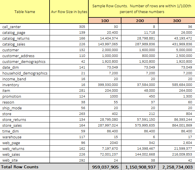
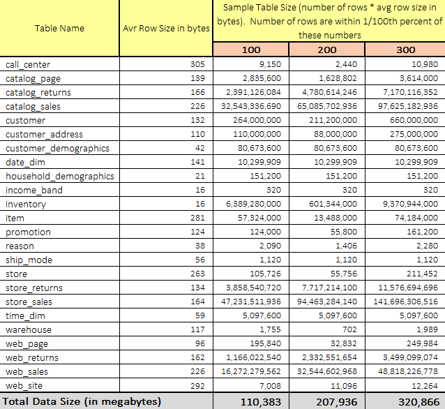
There are quite a few data sets and methodologies that can be used to gauge data storage and processing system’s performance e.g. TLC Trip Record Data released by the New York City Taxi & Limousine Commission has gained a lot of traction amongst big data specialists, however, TPC-approved benchmarks have long been considered as the most objective, vendor-agnostic way to perform data-specific hardware and software comparisons, capturing the complexity of modern business processing to a much greater extent than its predecessors. I have briefly outlined data generation mechanism used in the TPC-DS suite of tools in my previous blog HERE so I will skip the details and use three previously generated datasets for this demo – one with the scaling factor of 100 (~100GB), one with the scaling factor of 200 (~200GB) and another with the scaling factor of 300 (~300GB). All three datasets have not turned out to be perfectly uniform in terms of expected rows count (presumably due to selecting the unsupported scaling factors), with large deviations recorded across some files e.g. ‘inventory’ table containing fewer records in 200GB dataset than in the 100GB one. However, the three datasets were quite linear in terms of raw data volume increases which was also reflected in runtimes across number of subsequent queries.
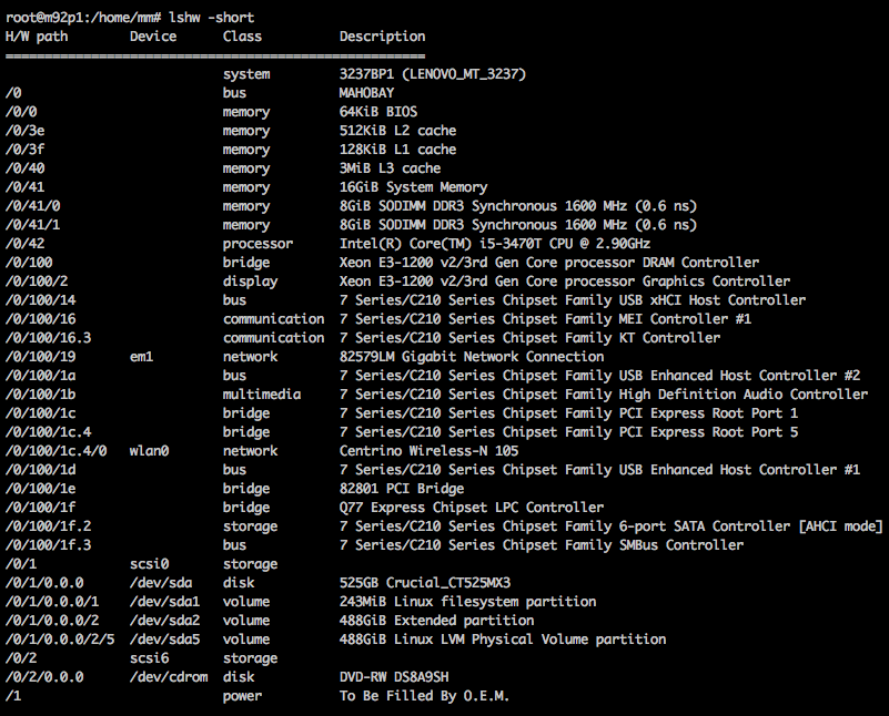
As mentioned in Post 2, the hardware used for this demo is not exactly what you would have in mind when provisioning an enterprise-class database cluster. With that in mind, the results of all the analytical queries I run are only indicative of the performance level in the context of the same data and configuration used. Chances are that with a proper, server-level hardware this comparison would be like going from the Wright brothers first airplane to Starship Enterprise but at least I endeavoured to make this as empirical as possible. To be completely transparent, here is the view of how these tiny Lenovo desktops are configured.
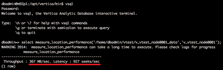
Also, for good measure I run a quick test on the storage performance using the ‘measure_locatioon_performance’ vsql function run on one of the machines (all three nodes are identical in terms of the individual components setup). These units are equipped with an SSD each (as opposed to a slower mechanical drive), however, their SATA2 interface limits the transfer rates of what these Crucial MX300 are technically capable of to just over 360 MB/sec as per the image below.
Finally, the fact I’m pushing between 100 and 300 gigabytes of data through this cluster with only 16GB of memory available per node means that most of the data needs to be read from disk. Most analytical databases are designed to cache data in memory, providing minimal latency and fast response time. As this hardware does not do justice to the data volumes queried in this demo, with proper reference architecture for this type of system I am certain that the performance would increase by an order of magnitude.
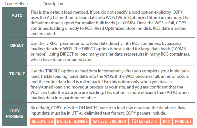
Vertica documentation provides a detail outline of different techniques used to load, transform and monitor the acquisitions. As reiterating the details of all the options and approaches is outside the scope of this post, I will only touch on some of the core concepts – for a comprehensive guide on data loading best practices and different options available please refer to their documentation or THIS visual guide. By far, the most effective way to load the data into Vertica is using COPY command. The COPY statement loads data from a file stored on the host or client (or in a data stream) into a database table. You can pass the COPY statement many different parameters to define various options such as: the format of the incoming data, metadata about the data load, which parser COPY should use, how to transform data as it is loaded or how to handle errors. Vertica’s hybrid storage model provides a great deal of flexibility for loading and managing data.
For this demo I copied and staged the three data sets – 100GB, 200GB and 300GB – on the m92p1 host (node no1 in my makeshift 3-node cluster) and used the following shell script to (1) create necessary tables on the previously created ‘vtest’ database and ‘tpc_ds’ schema and (2) load the data into the newly created tables.
#!/bin/bash
VPASS="YourPassword"
DBNAME="vtest"
SCHEMANAME="tpc_ds"
DATAFILEPATH="/home/dbadmin/vertica_stuff/TPC_DS_Data/100GB/*.dat"
SQLFILEPATH="/home/dbadmin/vertica_stuff/TPC_DS_SQL/create_pgsql_tables.sql"

/opt/vertica/bin/vsql -f "$SQLFILEPATH" -U dbadmin -w $VPASS -d $DBNAME
for file in $DATAFILEPATH
do
    filename=$(basename "$file")
    tblname=$(basename "$file" | cut -f 1 -d '.')
    echo "Loading file "$filename" into a Vertica host..."
    #single node only:
    echo "COPY $SCHEMANAME.$tblname FROM LOCAL '/home/dbadmin/vertica_stuff/TPC_DS_Data/100GB/$filename' \
        DELIMITER '|' DIRECT;" | \
         /opt/vertica/bin/vsql \
         -U dbadmin \
         -w $VPASS \
         -d $DBNAME
done
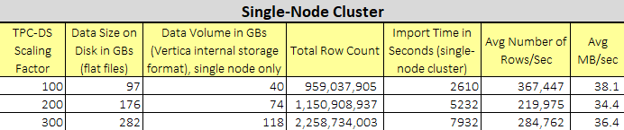
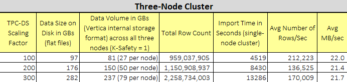
The sql file with all the DDL statements for tables’ creation can be downloaded from my OneDrive folder HERE. The script loaded the data using DIRECT option thus straight into ROS (Read Optimised Store) to avoid engaging the Tuple Mover – database optimiser component that moves data from memory (WOS) to disk (ROS). The load times (1000 Mbps Ethernet), along with some other supporting information, for each of the three datasets are listed below.
Testing Methodology and Results
A full TPC-DS benchmark is comprised of 99 queries and governed by very specific set of rules. For brevity, this demo only includes 20 queries i.e. (query number 5, 9, 10, 13, 17, 24, 31, 33, 34, 35, 44, 46, 47, 54, 57, 64, 74, 75, 97 and 99) as a subset sample for two reasons.
- The hardware, database setup, data volumes etc. analysed does not follow the characteristics and requirements outline by the TPC organisation and under these circumstances would be considered an ‘unacceptable consideration’. For example, a typical benchmark submitted by a vendor needs to include a number of metrics beyond query throughput e.g. a price-performance ratio, data load times, the availability date of the complete configuration etc. The following is a sample of a compliant reporting of TPC-DS results: ‘At 10GB the RALF/3000 Server has a TPC-DS Query-per-Hour metric of 3010 when run against a 10GB database yielding a TPC-DS Price/Performance of $1,202 per query-per-hour and will be available 1-Apr-06’. As this demo and the results below go only skin-deep i.e. query execution times, as previously stated, are only indicative of the performance level in the context of the same data and configuration used, enterprise-ready deployment would yield different (better) results.
- As this post is just for fun more than science, running 20 queries seems adequate enough to gauge the performance level dichotomies between the single and the multi-cluster environments.
Also, it is worth mentioning that no performance optimisation (database or OS level) was performed on the system. Vertica allows its administrator(s) to fine-tune various aspects of its operation through mechanisms such as statistics update, table partitioning, creating query or workload-specific projections, tuning execution plans etc. Some of those techniques require a deep knowledge of Vertica’s query execution engine while others can be achieved with little effort e.g. running DBD (Database Designer) – a GUI based tool which analyses the logical schema definition, sample data, and sample queries, and creates a physical schema in the form of a SQL script that you deploy automatically. While the initial scope of this series was intended to compare queries execution times across both versions (tuned and untuned), given the fact that Vertica’s is purposefully suited to run on a cluster of hosts, I decided to focus on contrasting single vs multi-node cluster deployment instead. Therefore, the results are only indicative of the performance level in the context of the same data and configuration used, with a good chance that further tuning, tweaking or other optimisation techniques would have yielded a much better performance outcomes.
OK, now with this little declaimer out of the way let’s look at how the first ten queries performed across the two distinct setups i.e. single node cluster and multi-node (3 nodes) cluster. Additional queries’ results as well as a quick look at a Tableau and PowerBI performance please refer to Part 4 of this series.
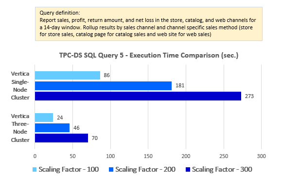
--Query 5
WITH ssr AS
(
         SELECT   s_store_id,
                  Sum(sales_price) AS sales,
                  Sum(profit)      AS profit,
                  Sum(return_amt)  AS returns1,
                  Sum(net_loss)    AS profit_loss
         FROM     (
                         SELECT ss_store_sk             AS store_sk,
                                ss_sold_date_sk         AS date_sk,
                                ss_ext_sales_price      AS sales_price,
                                ss_net_profit           AS profit,
                                Cast(0 AS DECIMAL(7,2)) AS return_amt,
                                Cast(0 AS DECIMAL(7,2)) AS net_loss
                         FROM   tpc_ds.store_sales
                         UNION ALL
                         SELECT sr_store_sk             AS store_sk,
                                sr_returned_date_sk     AS date_sk,
                                Cast(0 AS DECIMAL(7,2)) AS sales_price,
                                Cast(0 AS DECIMAL(7,2)) AS profit,
                                sr_return_amt           AS return_amt,
                                sr_net_loss             AS net_loss
                         FROM   tpc_ds.store_returns ) salesreturns,
                  tpc_ds.date_dim,
                  tpc_ds.store
         WHERE    date_sk = d_date_sk
         AND      d_date BETWEEN Cast('2002-08-22' AS DATE) AND      (
                           Cast('2002-08-22' AS DATE) + INTERVAL '14' day)
         AND      store_sk = s_store_sk
         GROUP BY s_store_id) , csr AS
(
         SELECT   cp_catalog_page_id,
                  sum(sales_price) AS sales,
                  sum(profit)      AS profit,
                  sum(return_amt)  AS returns1,
                  sum(net_loss)    AS profit_loss
         FROM     (
                         SELECT cs_catalog_page_sk      AS page_sk,
                                cs_sold_date_sk         AS date_sk,
                                cs_ext_sales_price      AS sales_price,
                                cs_net_profit           AS profit,
                                cast(0 AS decimal(7,2)) AS return_amt,
                                cast(0 AS decimal(7,2)) AS net_loss
                         FROM   tpc_ds.catalog_sales
                         UNION ALL
                         SELECT cr_catalog_page_sk      AS page_sk,
                                cr_returned_date_sk     AS date_sk,
                                cast(0 AS decimal(7,2)) AS sales_price,
                                cast(0 AS decimal(7,2)) AS profit,
                                cr_return_amount        AS return_amt,
                                cr_net_loss             AS net_loss
                         FROM   tpc_ds.catalog_returns ) salesreturns,
                  tpc_ds.date_dim,
                  tpc_ds.catalog_page
         WHERE    date_sk = d_date_sk
         AND      d_date BETWEEN cast('2002-08-22' AS date) AND      (
                           cast('2002-08-22' AS date) + INTERVAL '14' day)
         AND      page_sk = cp_catalog_page_sk
         GROUP BY cp_catalog_page_id) , wsr AS
(
         SELECT   web_site_id,
                  sum(sales_price) AS sales,
                  sum(profit)      AS profit,
                  sum(return_amt)  AS returns1,
                  sum(net_loss)    AS profit_loss
         FROM     (
                         SELECT ws_web_site_sk          AS wsr_web_site_sk,
                                ws_sold_date_sk         AS date_sk,
                                ws_ext_sales_price      AS sales_price,
                                ws_net_profit           AS profit,
                                cast(0 AS decimal(7,2)) AS return_amt,
                                cast(0 AS decimal(7,2)) AS net_loss
                         FROM   tpc_ds.web_sales
                         UNION ALL
                         SELECT          ws_web_site_sk          AS wsr_web_site_sk,
                                         wr_returned_date_sk     AS date_sk,
                                         cast(0 AS decimal(7,2)) AS sales_price,
                                         cast(0 AS decimal(7,2)) AS profit,
                                         wr_return_amt           AS return_amt,
                                         wr_net_loss             AS net_loss
                         FROM            tpc_ds.web_returns
                         LEFT OUTER JOIN tpc_ds.web_sales
                         ON              (
                                                         wr_item_sk = ws_item_sk
                                         AND             wr_order_number = ws_order_number) ) salesreturns,
                  tpc_ds.date_dim,
                  tpc_ds.web_site
         WHERE    date_sk = d_date_sk
         AND      d_date BETWEEN cast('2002-08-22' AS date) AND      (
                           cast('2002-08-22' AS date) + INTERVAL '14' day)
         AND      wsr_web_site_sk = web_site_sk
         GROUP BY web_site_id)
SELECT
         channel ,
         id ,
         sum(sales)   AS sales ,
         sum(returns1) AS returns1 ,
         sum(profit)  AS profit
FROM     (
                SELECT 'store channel' AS channel ,
                       'store'
                              || s_store_id AS id ,
                       sales ,
                       returns1 ,
                       (profit - profit_loss) AS profit
                FROM   ssr
                UNION ALL
                SELECT 'catalog channel' AS channel ,
                       'catalog_page'
                              || cp_catalog_page_id AS id ,
                       sales ,
                       returns1 ,
                       (profit - profit_loss) AS profit
                FROM   csr
                UNION ALL
                SELECT 'web channel' AS channel ,
                       'web_site'
                              || web_site_id AS id ,
                       sales ,
                       returns1 ,
                       (profit - profit_loss) AS profit
                FROM   wsr ) x
GROUP BY rollup (channel, id)
ORDER BY channel ,
         id
LIMIT 100;
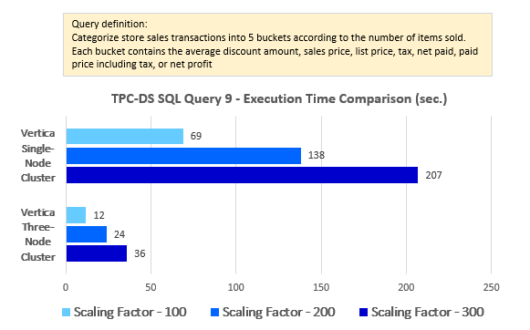
--Query 9
SELECT CASE
         WHEN (SELECT Count(*)
               FROM   tpc_ds.store_sales
               WHERE  ss_quantity BETWEEN 1 AND 20) > 3672 THEN
         (SELECT Avg(ss_ext_list_price)
          FROM   tpc_ds.store_sales
          WHERE
         ss_quantity BETWEEN 1 AND 20)
         ELSE (SELECT Avg(ss_net_profit)
               FROM   tpc_ds.store_sales
               WHERE  ss_quantity BETWEEN 1 AND 20)
       END bucket1,
       CASE
         WHEN (SELECT Count(*)
               FROM   tpc_ds.store_sales
               WHERE  ss_quantity BETWEEN 21 AND 40) > 3392 THEN
         (SELECT Avg(ss_ext_list_price)
          FROM   tpc_ds.store_sales
          WHERE
         ss_quantity BETWEEN 21 AND 40)
         ELSE (SELECT Avg(ss_net_profit)
               FROM   tpc_ds.store_sales
               WHERE  ss_quantity BETWEEN 21 AND 40)
       END bucket2,
       CASE
         WHEN (SELECT Count(*)
               FROM   tpc_ds.store_sales
               WHERE  ss_quantity BETWEEN 41 AND 60) > 32784 THEN
         (SELECT Avg(ss_ext_list_price)
          FROM   tpc_ds.store_sales
          WHERE
         ss_quantity BETWEEN 41 AND 60)
         ELSE (SELECT Avg(ss_net_profit)
               FROM   tpc_ds.store_sales
               WHERE  ss_quantity BETWEEN 41 AND 60)
       END bucket3,
       CASE
         WHEN (SELECT Count(*)
               FROM   tpc_ds.store_sales
               WHERE  ss_quantity BETWEEN 61 AND 80) > 26032 THEN
         (SELECT Avg(ss_ext_list_price)
          FROM   tpc_ds.store_sales
          WHERE
         ss_quantity BETWEEN 61 AND 80)
         ELSE (SELECT Avg(ss_net_profit)
               FROM   tpc_ds.store_sales
               WHERE  ss_quantity BETWEEN 61 AND 80)
       END bucket4,
       CASE
         WHEN (SELECT Count(*)
               FROM   tpc_ds.store_sales
               WHERE  ss_quantity BETWEEN 81 AND 100) > 23982 THEN
         (SELECT Avg(ss_ext_list_price)
          FROM   tpc_ds.store_sales
          WHERE
         ss_quantity BETWEEN 81 AND 100)
         ELSE (SELECT Avg(ss_net_profit)
               FROM   tpc_ds.store_sales
               WHERE  ss_quantity BETWEEN 81 AND 100)
       END bucket5
FROM   tpc_ds.reason
WHERE  r_reason_sk = 1;
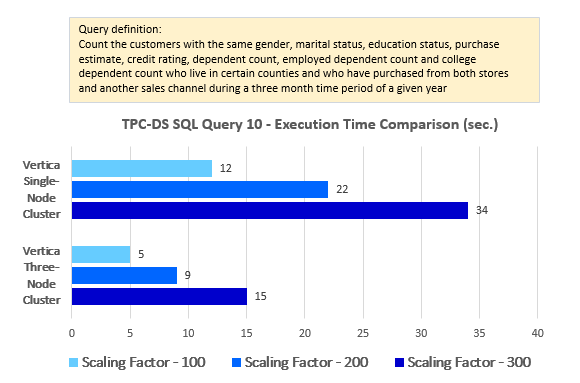
--Query 10
SELECT cd_gender,
               cd_marital_status,
               cd_education_status,
               Count(*) cnt1,
               cd_purchase_estimate,
               Count(*) cnt2,
               cd_credit_rating,
               Count(*) cnt3,
               cd_dep_count,
               Count(*) cnt4,
               cd_dep_employed_count,
               Count(*) cnt5,
               cd_dep_college_count,
               Count(*) cnt6
FROM   tpc_ds.customer c,
       tpc_ds.customer_address ca,
       tpc_ds.customer_demographics
WHERE  c.c_current_addr_sk = ca.ca_address_sk
       AND ca_county IN ( 'Lycoming County', 'Sheridan County',
                          'Kandiyohi County',
                          'Pike County',
                                           'Greene County' )
       AND cd_demo_sk = c.c_current_cdemo_sk
       AND EXISTS (SELECT *
                   FROM   tpc_ds.store_sales,
                          tpc_ds.date_dim
                   WHERE  c.c_customer_sk = ss_customer_sk
                          AND ss_sold_date_sk = d_date_sk
                          AND d_year = 2002
                          AND d_moy BETWEEN 4 AND 4 + 3)
       AND ( EXISTS (SELECT *
                     FROM   tpc_ds.web_sales,
                            tpc_ds.date_dim
                     WHERE  c.c_customer_sk = ws_bill_customer_sk
                            AND ws_sold_date_sk = d_date_sk
                            AND d_year = 2002
                            AND d_moy BETWEEN 4 AND 4 + 3)
              OR EXISTS (SELECT *
                         FROM   tpc_ds.catalog_sales,
                                tpc_ds.date_dim
                         WHERE  c.c_customer_sk = cs_ship_customer_sk
                                AND cs_sold_date_sk = d_date_sk
                                AND d_year = 2002
                                AND d_moy BETWEEN 4 AND 4 + 3) )
GROUP  BY cd_gender,
          cd_marital_status,
          cd_education_status,
          cd_purchase_estimate,
          cd_credit_rating,
          cd_dep_count,
          cd_dep_employed_count,
          cd_dep_college_count
ORDER  BY cd_gender,
          cd_marital_status,
          cd_education_status,
          cd_purchase_estimate,
          cd_credit_rating,
          cd_dep_count,
          cd_dep_employed_count,
          cd_dep_college_count
LIMIT 100;
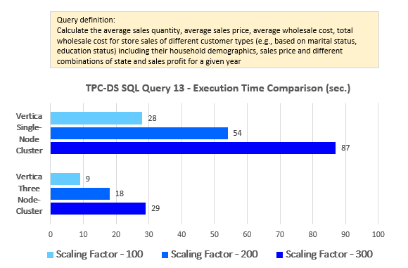
--Query 13
SELECT Avg(ss_quantity),
       Avg(ss_ext_sales_price),
       Avg(ss_ext_wholesale_cost),
       Sum(ss_ext_wholesale_cost)
FROM   tpc_ds.store_sales,
       tpc_ds.store,
       tpc_ds.customer_demographics,
       tpc_ds.household_demographics,
       tpc_ds.customer_address,
       tpc_ds.date_dim
WHERE  s_store_sk = ss_store_sk
       AND ss_sold_date_sk = d_date_sk
       AND d_year = 2001
       AND ( ( ss_hdemo_sk = hd_demo_sk
               AND cd_demo_sk = ss_cdemo_sk
               AND cd_marital_status = 'U'
               AND cd_education_status = 'Advanced Degree'
               AND ss_sales_price BETWEEN 100.00 AND 150.00
               AND hd_dep_count = 3 )
              OR ( ss_hdemo_sk = hd_demo_sk
                   AND cd_demo_sk = ss_cdemo_sk
                   AND cd_marital_status = 'M'
                   AND cd_education_status = 'Primary'
                   AND ss_sales_price BETWEEN 50.00 AND 100.00
                   AND hd_dep_count = 1 )
              OR ( ss_hdemo_sk = hd_demo_sk
                   AND cd_demo_sk = ss_cdemo_sk
                   AND cd_marital_status = 'D'
                   AND cd_education_status = 'Secondary'
                   AND ss_sales_price BETWEEN 150.00 AND 200.00
                   AND hd_dep_count = 1 ) )
       AND ( ( ss_addr_sk = ca_address_sk
               AND ca_country = 'United States'
               AND ca_state IN ( 'AZ', 'NE', 'IA' )
               AND ss_net_profit BETWEEN 100 AND 200 )
              OR ( ss_addr_sk = ca_address_sk
                   AND ca_country = 'United States'
                   AND ca_state IN ( 'MS', 'CA', 'NV' )
                   AND ss_net_profit BETWEEN 150 AND 300 )
              OR ( ss_addr_sk = ca_address_sk
                   AND ca_country = 'United States'
                   AND ca_state IN ( 'GA', 'TX', 'NJ' )
                   AND ss_net_profit BETWEEN 50 AND 250 ) );
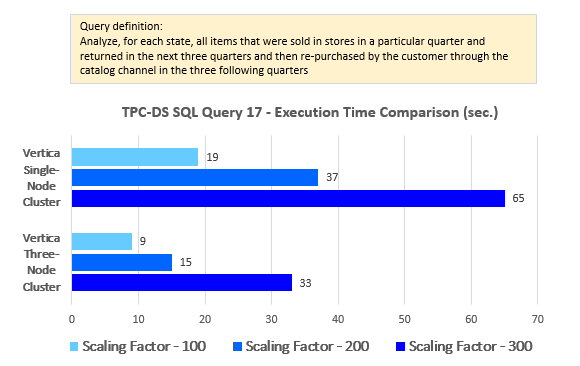
--Query 17
SELECT i_item_id,
               i_item_desc,
               s_state,
               Count(ss_quantity)                                        AS
               store_sales_quantitycount,
               Avg(ss_quantity)                                          AS
               store_sales_quantityave,
               Stddev_samp(ss_quantity)                                  AS
               store_sales_quantitystdev,
               Stddev_samp(ss_quantity) / Avg(ss_quantity)               AS
               store_sales_quantitycov,
               Count(sr_return_quantity)                                 AS
               store_returns_quantitycount,
               Avg(sr_return_quantity)                                   AS
               store_returns_quantityave,
               Stddev_samp(sr_return_quantity)                           AS
               store_returns_quantitystdev,
               Stddev_samp(sr_return_quantity) / Avg(sr_return_quantity) AS
               store_returns_quantitycov,
               Count(cs_quantity)                                        AS
               catalog_sales_quantitycount,
               Avg(cs_quantity)                                          AS
               catalog_sales_quantityave,
               Stddev_samp(cs_quantity) / Avg(cs_quantity)               AS
               catalog_sales_quantitystdev,
               Stddev_samp(cs_quantity) / Avg(cs_quantity)               AS
               catalog_sales_quantitycov
FROM   tpc_ds.store_sales,
       tpc_ds.store_returns,
       tpc_ds.catalog_sales,
       tpc_ds.date_dim d1,
       tpc_ds.date_dim d2,
       tpc_ds.date_dim d3,
       tpc_ds.store,
       tpc_ds.item
WHERE  d1.d_quarter_name = '1999Q1'
       AND d1.d_date_sk = ss_sold_date_sk
       AND i_item_sk = ss_item_sk
       AND s_store_sk = ss_store_sk
       AND ss_customer_sk = sr_customer_sk
       AND ss_item_sk = sr_item_sk
       AND ss_ticket_number = sr_ticket_number
       AND sr_returned_date_sk = d2.d_date_sk
       AND d2.d_quarter_name IN ( '1999Q1', '1999Q2', '1999Q3' )
       AND sr_customer_sk = cs_bill_customer_sk
       AND sr_item_sk = cs_item_sk
       AND cs_sold_date_sk = d3.d_date_sk
       AND d3.d_quarter_name IN ( '1999Q1', '1999Q2', '1999Q3' )
GROUP  BY i_item_id,
          i_item_desc,
          s_state
ORDER  BY i_item_id,
          i_item_desc,
          s_state
LIMIT 100;
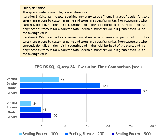
--Query 24
WITH ssales
     AS (SELECT c_last_name,
                c_first_name,
                s_store_name,
                ca_state,
                s_state,
                i_color,
                i_current_price,
                i_manager_id,
                i_units,
                i_size,
                Sum(ss_net_profit) netpaid
         FROM   tpc_ds.store_sales,
                tpc_ds.store_returns,
                tpc_ds.store,
                tpc_ds.item,
                tpc_ds.customer,
                tpc_ds.customer_address
         WHERE  ss_ticket_number = sr_ticket_number
                AND ss_item_sk = sr_item_sk
                AND ss_customer_sk = c_customer_sk
                AND ss_item_sk = i_item_sk
                AND ss_store_sk = s_store_sk
                AND c_birth_country = Upper(ca_country)
                AND s_zip = ca_zip
                AND s_market_id = 6
         GROUP  BY c_last_name,
                   c_first_name,
                   s_store_name,
                   ca_state,
                   s_state,
                   i_color,
                   i_current_price,
                   i_manager_id,
                   i_units,
                   i_size)
SELECT c_last_name,
       c_first_name,
       s_store_name,
       Sum(netpaid) paid
FROM   ssales
WHERE  i_color = 'papaya'
GROUP  BY c_last_name,
          c_first_name,
          s_store_name
HAVING Sum(netpaid) > (SELECT 0.05 * Avg(netpaid)
                       FROM   ssales);

WITH ssales
     AS (SELECT c_last_name,
                c_first_name,
                s_store_name,
                ca_state,
                s_state,
                i_color,
                i_current_price,
                i_manager_id,
                i_units,
                i_size,
                Sum(ss_net_profit) netpaid
         FROM   tpc_ds.store_sales,
                tpc_ds.store_returns,
                tpc_ds.store,
                tpc_ds.item,
                tpc_ds.customer,
                tpc_ds.customer_address
         WHERE  ss_ticket_number = sr_ticket_number
                AND ss_item_sk = sr_item_sk
                AND ss_customer_sk = c_customer_sk
                AND ss_item_sk = i_item_sk
                AND ss_store_sk = s_store_sk
                AND c_birth_country = Upper(ca_country)
                AND s_zip = ca_zip
                AND s_market_id = 6
         GROUP  BY c_last_name,
                   c_first_name,
                   s_store_name,
                   ca_state,
                   s_state,
                   i_color,
                   i_current_price,
                   i_manager_id,
                   i_units,
                   i_size)
SELECT c_last_name,
       c_first_name,
       s_store_name,
       Sum(netpaid) paid
FROM   ssales
WHERE  i_color = 'chartreuse'
GROUP  BY c_last_name,
          c_first_name,
          s_store_name
HAVING Sum(netpaid) > (SELECT 0.05 * Avg(netpaid)
                       FROM   ssales);
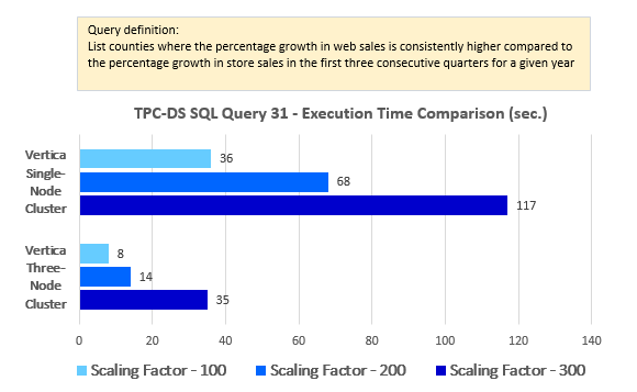
--Query 31
WITH ss
     AS (SELECT ca_county,
                d_qoy,
                d_year,
                Sum(ss_ext_sales_price) AS store_sales
         FROM   tpc_ds.store_sales,
                tpc_ds.date_dim,
                tpc_ds.customer_address
         WHERE  ss_sold_date_sk = d_date_sk
                AND ss_addr_sk = ca_address_sk
         GROUP  BY ca_county,
                   d_qoy,
                   d_year),
     ws
     AS (SELECT ca_county,
                d_qoy,
                d_year,
                Sum(ws_ext_sales_price) AS web_sales
         FROM   tpc_ds.web_sales,
                tpc_ds.date_dim,
                tpc_ds.customer_address
         WHERE  ws_sold_date_sk = d_date_sk
                AND ws_bill_addr_sk = ca_address_sk
         GROUP  BY ca_county,
                   d_qoy,
                   d_year)
SELECT ss1.ca_county,
       ss1.d_year,
       ws2.web_sales / ws1.web_sales     web_q1_q2_increase,
       ss2.store_sales / ss1.store_sales store_q1_q2_increase,
       ws3.web_sales / ws2.web_sales     web_q2_q3_increase,
       ss3.store_sales / ss2.store_sales store_q2_q3_increase
FROM   ss ss1,
       ss ss2,
       ss ss3,
       ws ws1,
       ws ws2,
       ws ws3
WHERE  ss1.d_qoy = 1
       AND ss1.d_year = 2001
       AND ss1.ca_county = ss2.ca_county
       AND ss2.d_qoy = 2
       AND ss2.d_year = 2001
       AND ss2.ca_county = ss3.ca_county
       AND ss3.d_qoy = 3
       AND ss3.d_year = 2001
       AND ss1.ca_county = ws1.ca_county
       AND ws1.d_qoy = 1
       AND ws1.d_year = 2001
       AND ws1.ca_county = ws2.ca_county
       AND ws2.d_qoy = 2
       AND ws2.d_year = 2001
       AND ws1.ca_county = ws3.ca_county
       AND ws3.d_qoy = 3
       AND ws3.d_year = 2001
       AND CASE
             WHEN ws1.web_sales > 0 THEN ws2.web_sales / ws1.web_sales
             ELSE NULL
           END > CASE
                   WHEN ss1.store_sales > 0 THEN
                   ss2.store_sales / ss1.store_sales
                   ELSE NULL
                 END
       AND CASE
             WHEN ws2.web_sales > 0 THEN ws3.web_sales / ws2.web_sales
             ELSE NULL
           END > CASE
                   WHEN ss2.store_sales > 0 THEN
                   ss3.store_sales / ss2.store_sales
                   ELSE NULL
                 END
ORDER  BY ss1.d_year;
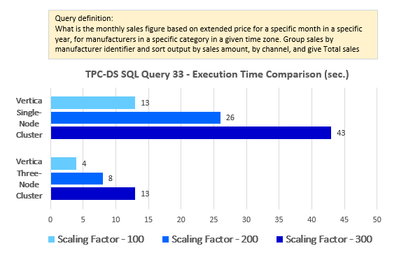
--Query 33
WITH ss
     AS (SELECT i_manufact_id,
                Sum(ss_ext_sales_price) total_sales
         FROM   tpc_ds.store_sales,
                tpc_ds.date_dim,
                tpc_ds.customer_address,
                tpc_ds.item
         WHERE  i_manufact_id IN (SELECT i_manufact_id
                                  FROM   tpc_ds.item
                                  WHERE  i_category IN ( 'Books' ))
                AND ss_item_sk = i_item_sk
                AND ss_sold_date_sk = d_date_sk
                AND d_year = 1999
                AND d_moy = 3
                AND ss_addr_sk = ca_address_sk
                AND ca_gmt_offset = -5
         GROUP  BY i_manufact_id),
     cs
     AS (SELECT i_manufact_id,
                Sum(cs_ext_sales_price) total_sales
         FROM   tpc_ds.catalog_sales,
                tpc_ds.date_dim,
                tpc_ds.customer_address,
                tpc_ds.item
         WHERE  i_manufact_id IN (SELECT i_manufact_id
                                  FROM   tpc_ds.item
                                  WHERE  i_category IN ( 'Books' ))
                AND cs_item_sk = i_item_sk
                AND cs_sold_date_sk = d_date_sk
                AND d_year = 1999
                AND d_moy = 3
                AND cs_bill_addr_sk = ca_address_sk
                AND ca_gmt_offset = -5
         GROUP  BY i_manufact_id),
     ws
     AS (SELECT i_manufact_id,
                Sum(ws_ext_sales_price) total_sales
         FROM   tpc_ds.web_sales,
                tpc_ds.date_dim,
                tpc_ds.customer_address,
                tpc_ds.item
         WHERE  i_manufact_id IN (SELECT i_manufact_id
                                  FROM   tpc_ds.item
                                  WHERE  i_category IN ( 'Books' ))
                AND ws_item_sk = i_item_sk
                AND ws_sold_date_sk = d_date_sk
                AND d_year = 1999
                AND d_moy = 3
                AND ws_bill_addr_sk = ca_address_sk
                AND ca_gmt_offset = -5
         GROUP  BY i_manufact_id)
SELECT i_manufact_id,
               Sum(total_sales) total_sales
FROM   (SELECT *
        FROM   ss
        UNION ALL
        SELECT *
        FROM   cs
        UNION ALL
        SELECT *
        FROM   ws) tmp1
GROUP  BY i_manufact_id
ORDER  BY total_sales
LIMIT 100;
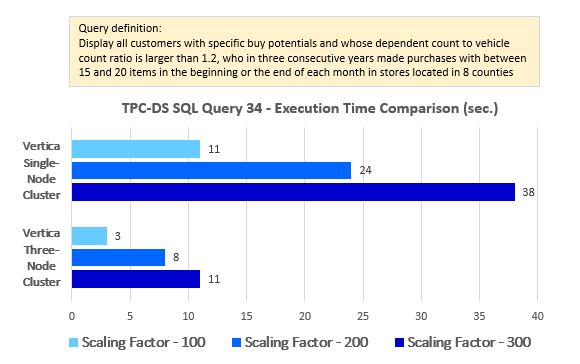
--Query 34
SELECT c_last_name,
       c_first_name,
       c_salutation,
       c_preferred_cust_flag,
       ss_ticket_number,
       cnt
FROM   (SELECT ss_ticket_number,
               ss_customer_sk,
               Count(*) cnt
        FROM   tpc_ds.store_sales,
               tpc_ds.date_dim,
               tpc_ds.store,
               tpc_ds.household_demographics
        WHERE  store_sales.ss_sold_date_sk = date_dim.d_date_sk
               AND store_sales.ss_store_sk = store.s_store_sk
               AND store_sales.ss_hdemo_sk = household_demographics.hd_demo_sk
               AND ( date_dim.d_dom BETWEEN 1 AND 3
                      OR date_dim.d_dom BETWEEN 25 AND 28 )
               AND ( household_demographics.hd_buy_potential = '>10000'
                      OR household_demographics.hd_buy_potential = 'unknown' )
               AND household_demographics.hd_vehicle_count > 0
               AND ( CASE
                       WHEN household_demographics.hd_vehicle_count > 0 THEN
                       household_demographics.hd_dep_count /
                       household_demographics.hd_vehicle_count
                       ELSE NULL
                     END ) > 1.2
               AND date_dim.d_year IN ( 1999, 1999 + 1, 1999 + 2 )
               AND store.s_county IN ( 'Williamson County', 'Williamson County',
                                       'Williamson County',
                                                             'Williamson County'
                                       ,
                                       'Williamson County', 'Williamson County',
                                           'Williamson County',
                                                             'Williamson County'
                                     )
        GROUP  BY ss_ticket_number,
                  ss_customer_sk) dn,
       tpc_ds.customer
WHERE  ss_customer_sk = c_customer_sk
       AND cnt BETWEEN 15 AND 20
ORDER  BY c_last_name,
          c_first_name,
          c_salutation,
          c_preferred_cust_flag DESC;
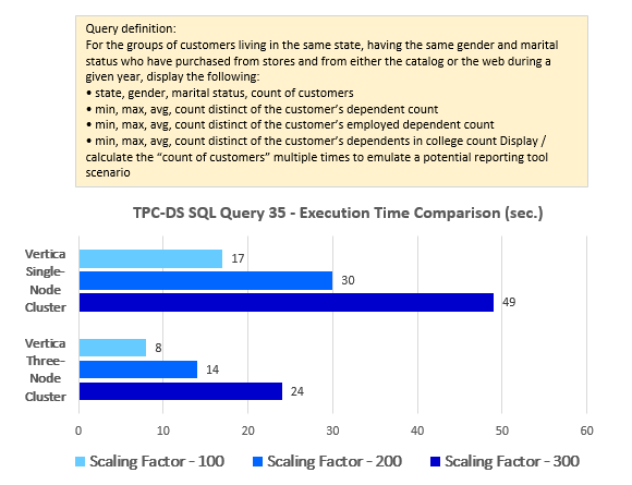
--Query 35
SELECT ca_state,
               cd_gender,
               cd_marital_status,
               cd_dep_count,
               Count(*) cnt1,
               Stddev_samp(cd_dep_count),
               Avg(cd_dep_count),
               Max(cd_dep_count),
               cd_dep_employed_count,
               Count(*) cnt2,
               Stddev_samp(cd_dep_employed_count),
               Avg(cd_dep_employed_count),
               Max(cd_dep_employed_count),
               cd_dep_college_count,
               Count(*) cnt3,
               Stddev_samp(cd_dep_college_count),
               Avg(cd_dep_college_count),
               Max(cd_dep_college_count)
FROM   tpc_ds.customer c,
       tpc_ds.customer_address ca,
       tpc_ds.customer_demographics
WHERE  c.c_current_addr_sk = ca.ca_address_sk
       AND cd_demo_sk = c.c_current_cdemo_sk
       AND EXISTS (SELECT *
                   FROM   tpc_ds.store_sales,
                          tpc_ds.date_dim
                   WHERE  c.c_customer_sk = ss_customer_sk
                          AND ss_sold_date_sk = d_date_sk
                          AND d_year = 2001
                          AND d_qoy < 4)
       AND ( EXISTS (SELECT *
                     FROM   tpc_ds.web_sales,
                            tpc_ds.date_dim
                     WHERE  c.c_customer_sk = ws_bill_customer_sk
                            AND ws_sold_date_sk = d_date_sk
                            AND d_year = 2001
                            AND d_qoy < 4)
              OR EXISTS (SELECT *
                         FROM   tpc_ds.catalog_sales,
                                tpc_ds.date_dim
                         WHERE  c.c_customer_sk = cs_ship_customer_sk
                                AND cs_sold_date_sk = d_date_sk
                                AND d_year = 2001
                                AND d_qoy < 4) )
GROUP  BY ca_state,
          cd_gender,
          cd_marital_status,
          cd_dep_count,
          cd_dep_employed_count,
          cd_dep_college_count
ORDER  BY ca_state,
          cd_gender,
          cd_marital_status,
          cd_dep_count,
          cd_dep_employed_count,
          cd_dep_college_count
LIMIT 100;
I decided to break up the queries’ performance analysis into two parts. Further TPC-DS queries’ results, along with a quick look at how Vertica plays with Tableau and PowerBI applications, can be viewed in Part 4 to this series but we can already see the execution pattern and how data volumes and its distribution across multiple nodes impact the performance. Again, please refer to Post 4 for data on the additional ten queries performance results and my final comments on this experiment.