bicortex

How To Build A Data Mart Using Microsoft BI Stack Part 5 – Defining SSAS Project And Its Dimensions

In the PREVIOUS POST I explored SQL Server Integration Services functionality and how the SQL code samples integrated into developing an ETL routine provide automated data mart loading. In this post I would like to start exploring the concept of using SQL Server Analysis Services as a storage engine for our dimensional data and how to start building a simple SSAS project with Data Source View and SASS dimensions defined.

Let’s open up BIDS or SQL Server Data Tools application (depending on which SQL Server version you’re using) and create an empty SSAS project. The first thing to do is to set up a data source connection. This is a wizard-driven task and we can execute it by right-clicking on Data Sources folder inside Solution Explorer pane and selection New Data Source from options provided. If you’re following along from PREVIOUS POST, a previously defined connection which we established in order to create our SSIS package should already be available to you. If not, please complete the wizard selecting DW_Sample database we create as our relational data mart for this project. Also, I recommend that you use Windows User Name and Password option when providing login credentials.

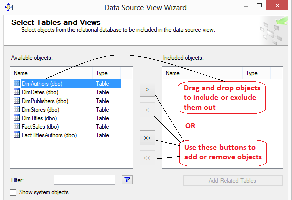
Next, it is time to create a data source view. Data source view (DSV) is a logic layer of abstraction consisting of table(s) with each table containing a saved SQL statement. It provides an interface and separation layer between relational database and cubes which can be very beneficial e.g. adjusting data model to fit the cube design without changing the underlying table structure. To start creating the DSV, right-click on Data Source View under Solution Explorer pane and select New Data Source View to kick off the wizard. Stepping through the wizard, after we selected the previously defined Data Source, we should be presented with Select Tables and Views pane as per image below.

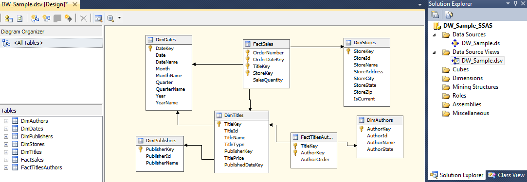
Let’s select all available objects i.e. two fact tables and five dimension tables by moving them from left-hand side to right-hand side by dragging and dropping or alternatively using  buttons between the two windows. On wizard completion we should be presented with a Data Source View table schema as our as per image below.

As we have foreign key constants already defined, the wizard automatically maps logical relationships between tables based on these constraints. If the constraints were missing, we would need to define them in a separate step. In the Data Source View Designer, both SQL Server tables and views are presented as tables. Each of those tables on the designer surface represents an underlying SQL select statement. For example, the DimAuthors table represents the following SQL statement: SELECT AuthorKey, AuthorId, AuthorName, AuthorState FROM DimAuthors. Analysis Services server uses these select statements to copy data into the cube.

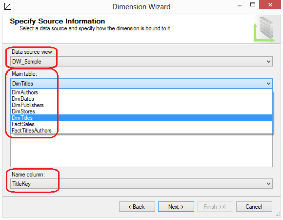
Next step is to define dimensions which describe attributes of measured values. In the DW_Sample_SSAS project, we currently have a single measure we need to describe: SalesQuantity. The SalesQuantity attributes are an order number, order date, title, and store. Accordingly, we create a dimension for each of these descriptors. To create a dimension, launch the Dimension Wizard by right-clicking the Dimensions folder in Solution Explorer and selecting New Dimension from the context menu. On screen number two called Create Creation Method let’s select Use an Existing Method option (as we already have fact and dimension tables defined in the database). Following on, we will specify Data Source View (we only have one in this project) and select a table from the Main Table dropdown box. Each dimension may have only one table, which of course will be its main table. In cases where the dimension is designed in a snowflake format, such as the Titles dimension in the DW_Sample_SSAS project, the main table is the one directly connected to the fact table. This means you do not have to select both the DimTitles table and the DimPublishers tables, only selecting the main DimTitles table as per image below.

Once you select a table, select one or more columns that define the table’s dimensional keys. Typically, they are singular key columns such as the TitleKey as per image above. If you have a composite key, you can select a second column by clicking the Add key column after you choose the initial key column. The last dropdown box on this page allows you to select a name column. The name column is the one that holds a label for the key column’s value. Clicking the Next button advances the wizard to one of two pages: the Dimension Attributes page or the Select Related Tables page. If the only relationship line you have in the data source view is to the fact table, you will advance to the Select Dimension Attributes page. If, however, you have tables in a snowflake pattern with relationship lines connecting to other dimensional tables, you will advance to the Select Related Tables page as per image below.

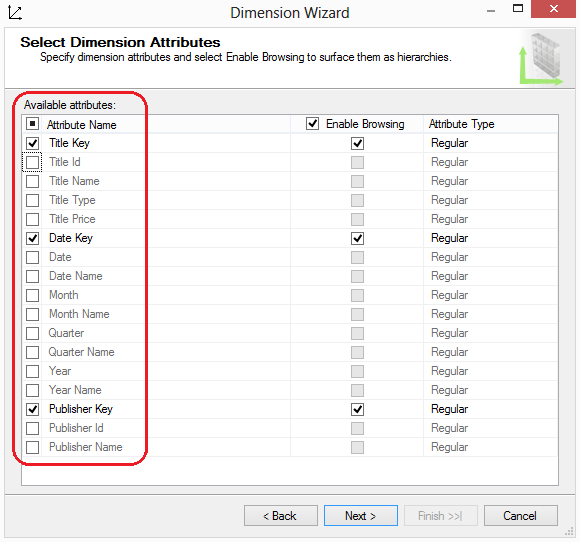
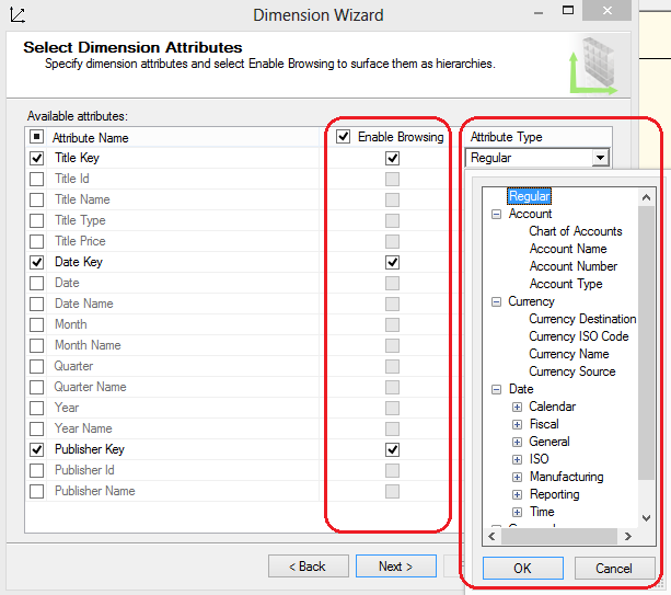
In our example, The DimTitles table is connected to both the DimPublishers and DimDates tables in the data source view. Therefore, the Select Related Tables page displays both of these tables with a checked checkbox. It is optional to include a related table; therefore, the wizard allows you to uncheck the checkbox if you feel a related table is not appropriate for the dimension you are currently building. In the case of the DimTitles table, we will leave both tables checked because they include additional information that we want to include as part of the Titles dimension. Next, on the Select Dimension Attributes page, you can choose to select all or some of the available attributes. In the current example, the DimTitles table relates to both the DimPublishers table and the DimDates table to form a snowflake design within the data source view. Because of this, we see many columns available from multiple dimensions in the Select Dimensional Attributes page as per image below.

It makes sense to include some of these columns from each dimension table, but not necessarily all of them. Including publishers’ names, for example, will allow for creating reports that can group titles by publishers. The same is true of the title types. But the artificial publisher key or the artificial date key (without an associated name column) is not as useful, because it is unlikely a report will benefit from either one of these columns. They have no significance outside the context of the data warehouse design. In the same step we can also define whether we permit the attribute to be visible to end users through Enable Browsing option and define the attribute type.

Most software ignores the Attribute Type setting; therefore, it has little to no impact on creating reports. Microsoft has included the setting for application programmed to use it, but leaving the selection at Regular is most often the appropriate choice. Occasionally an attribute’s type must be more definitive. For example, when the dimensional attribute includes date data, the attribute type should always be configured to reflect the content. The date data determines how SSAS performs aggregations and how MDX functions are processed. In our current example date, month, quarter, and year attributes must be configured accordingly. Once all parameters have been defined we can save the dimension with a new name and proceed to further configuration steps before we can deploy them.

In order to cut the number of steps and screenshots, I have put together this short document which takes each project dimension and configures its attributes. It has all the necessary steps to configure dimensions as per above recommendations and if you’re keen to follow along you can access/download it from HERE.

Believe or not, there is still quite some work to be done to configure the dimensions and fact tables in order to create an SSAS cube. In the NEXT PART to this series, I will go over some of the dimension properties and hierarchies that still require attention before explaining cube creation and deployment process.  As usual, the code used in this series as well as solution files for this SSAS project can be found and downloaded from HERE.

Please also check other posts from this series:

• How To Build A Data Mart Using Microsoft BI Stack Part 1 – Introduction and OLTP Database Analysis
• How To Build A Data Mart Using Microsoft BI Stack Part 2 – OLAP Database Objects Modelling
• How To Build A Data Mart Using Microsoft BI Stack Part 3 – Data Mart Load Approach And Coding
• How To Build A Data Mart Using Microsoft BI Stack Part 4 – Data Mart Load Using SSIS
• How To Build A Data Mart Using Microsoft BI Stack Part 6 – Refining SSAS Data Warehouse Dimensions
• How To Build A Data Mart Using Microsoft BI Stack Part 7 – Cube Creation, Cube Deployment And Data Validation
• How To Build A Data Mart Using Microsoft BI Stack Part 8 – Creating Sample SSRS Report

All SQL code and solution files can be found and downloaded from HERE.

http://scuttle.org/bookmarks.php/pass?action=add

Posted in: Data Modelling, How To's, SSAS

Tags: Data Modelling, SSAS

This entry was posted on Monday, September 16th, 2013 at 3:14 am and is filed under Data Modelling, How To's, SSAS. You can follow any responses to this entry through the RSS 2.0 feed. You can leave a response, or trackback from your own site.