Data Acquisition Framework Using Custom Python Wrapper For Concurrent BCP Utility Execution
October 2nd, 2018 / No Comments » / by admin
Although building a data acquisition framework for a data warehouse isn’t nearly or as interesting as doing analytics or data mining on the already well-structured data, it’s an essential part of any data warehousing project. I have already written extensively on how one could build a robust data acquisition framework in THIS series of blog posts, however, given the rapidly growing ecosystem of data sources and data stores, more and more projects tend to gravitate to the more application-agnostic storage formats e.g. text files or column-oriented files e.g. parquet. As such, direct data store connection may not be a possibility or the most optimal way of exporting data, making flat file export/import option a good alternative.
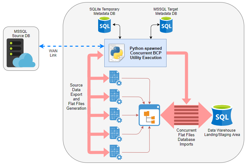
Microsoft offers a few different tools to facilitate flat files imports and exports, the most commonly used being bcp, BULK INSERT and their own ETL tool, capable of connecting to and reading flat files – SSIS. In this demo, I will analyse the difference in performance for data export and import between using pure T-SQL (executed as a series of concurrently running SQL Agent jobs) and parallelised bcp operations (using custom Python wrapper). Below image depicts high-level architecture of the solution with a short video clip demonstrating the actual code execution on a sample dataset at the end of this post. Let’s compare the pair and see if any of them is better at moving data across the wire.
Database and Schema Setup
Most of data warehouses come with some form of metadata layer so for this exercise I have ‘scrapped’ the source metadata e.g. attributes such as object names, data types, row counts etc. into a Sqlite local database. I also copied over partial target database metadata (with a bit more structure imposed) from one of the systems I’m currently working with. This resulted in creating the following schema of tables containing key information on source and target objects, their attributes, their state etc.
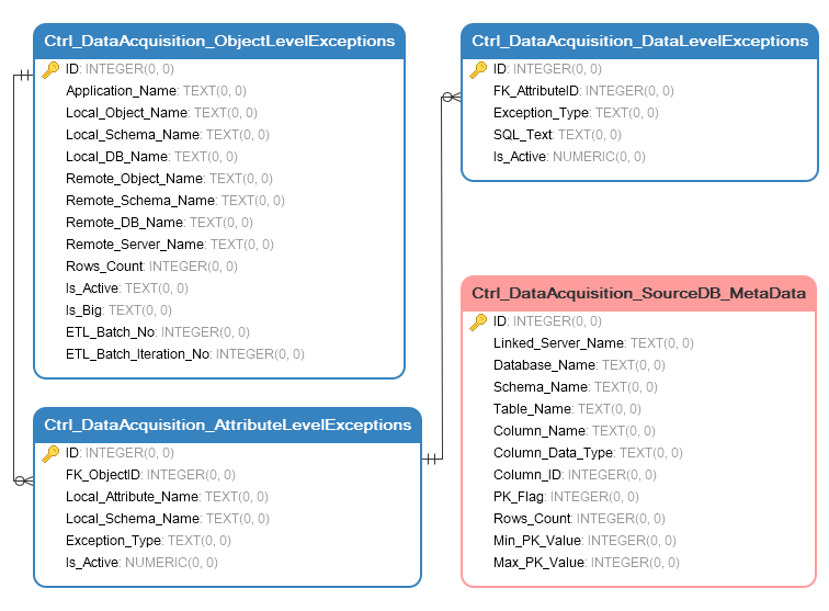
Target metadata is contained to three tables which allow for a three-layer, hierarchical approach to data acquisition:
- Ctrl_DataAcquisition_ObjectLevelExceptions table stores details of database objects with some other peripheral information. The grain of this table is set to the object (table) level which then allows for an easy object tagging and acquisitions inclusion/exclusion.
- Ctrl_DataAcquisition_AttributeLevelExceptions table stores attributes level data. It references ‘objects’ table and determines which fields out of the referenced object are to be included/excluded.
- Ctrl_DataAcquisition_DataLevelExceptions table stores any statements which need to be executed in order to remove/retain specific values.
As a result, thanks to this setup, we now have the option to dictate which objects are to be acquired, which fields from those objects are to be retained/omitted and finally which values out of these attributes are to be persisted/hashed/obfuscated/removed etc. Source-level metadata (in this scenario) was diluted to a single table containing some of the key attributes and data to fulfil the requirements for this post.
Creating the metadata repository, depending on the system’s complexity and level of detail required, can be quite challenging in itself so I will leave out the particulars out of this post, however, it’s important to note that this mini-framework would not be possible without storing and comparing both systems’ metadata i.e. source database and target database.
This post also scratches the surface of actual metadata layer implementation details but suffice to say that any well designed and architected framework should lean heavily on metadata. For this post, mainly to preserve the brevity and the focus on the problem analysed, I have obfuscated the details of target metadata creation and diluted source metadata ‘scrapping’ to bare minimum.
The key information sourced, aside from which tables and columns to handle, is essential to providing a more flexible approach to data extraction for the following reasons:
- Primary key flag – identifies a specific attribute as either a primary key or not a primary key in order to split a large table into multiple ‘chunks’. As most primary keys are of data type INTEGER (or its derivative e.g. SMALLINT, TINYINT, BIGINT) splitting larger tables into smaller streams of data and files allows for better resources utilisation.
- Column data type – useful in checking whether arithmetic can be performed on the given table’s primary key i.e. if it’s not an INTEGER (or similar) than subdividing into smaller partitions will not be an option.
- Rows count – this data is required I order to partition larger tables into smaller shards based on the total record count.
- Minimum record count – this value is essential for partitioning larger tables which do not have their seeding values starting from one.
- Maximum record count – same as above, this piece of data is required to ascertain the ceiling value for further data ‘chunking’.
The following Python script was used to create and populate MetadataDB.db database.
import configparser
import sqlite3
import os
import sys
import pyodbc


config = configparser.ConfigParser()
config.read("params.cfg")

dbsqlite_location = config.get("Sqlite", os.path.normpath("dbsqlite_location"))
dbsqlite_fileName = config.get("Sqlite", "dbsqlite_fileName")
dbsqlite_sql = config.get("Sqlite", "dbsqlite_sql")
dbsqlite_import_tables = config.get("Tables_To_Import", "local_mssql_meta_tables")
dbsqlite_import_tables = dbsqlite_import_tables.split(",")
dbsqlite_excluded_attribs = config.get("Tables_To_Import", "local_mssql_meta_attributes_to_exclude")
dbsqlite_excluded_attribs = dbsqlite_excluded_attribs.split(",")
dbsqlite_import_tables_remote = config.get("Tables_To_Import", "remote_meta_tables")


def get_sql(dbsqlite_location, dbsqlite_fileName, dbsqlite_sql):
    """
    Source operation types from the SQL file - denoted by the use of four dash characteres
    and store them in a dictionary (referenced later)
    """
    if os.path.isfile(dbsqlite_fileName):
        os.remove(dbsqlite_fileName)
    operations = []
    commands = []

    with open(dbsqlite_sql, "r") as f:
        for i in f:
            if i.startswith("----"):
                i = i.replace("----", "")
                operations.append(i.rstrip("\n"))

    tempCommands = []
    with open(dbsqlite_sql, "r") as f:
        for i in f:
            tempCommands.append(i)
        l = [i for i, s in enumerate(tempCommands) if "----" in s]
        l.append((len(tempCommands)))
        for first, second in zip(l, l[1:]):
            commands.append("".join(tempCommands[first:second]))
    sql = dict(zip(operations, commands))
    return sql


def build_db(dbsqlite_location, dbsqlite_fileName, sql):
    """
    Build the database
    """
    print("Building TableauEX.db database schema... ")
    with sqlite3.connect(
        os.path.join(dbsqlite_location, dbsqlite_fileName)
    ) as sqlLiteConn:
        sqlCommands = sql.get("SQL 1: Build_Meta_DB").split(";")
        for c in sqlCommands:
            try:
                sqlLiteConn.execute(c)
            except Exception as e:
                print(e)
                sqlLiteConn.rollback()
                sys.exit(1)
            else:
                sqlLiteConn.commit()


def populate_db_from_mssql_meta(
    dbsqlite_import_tables, dbsqlite_excluded_attribs, sql, **options
):
    """
    Source local instance MSSQL metadata
    and populate Sqlite tables with the data.
    """
    mssql_args = {
        "Driver": options.get("Driver", "ODBC Driver 13 for SQL Server"),
        "Server": options.get("Server", "ServerName\\InstanceName"),
        "Database": options.get("Database", "Metadata_DB_Name"),
        "Trusted_Connection": options.get("Trusted_Connection", "yes"),
    }

    cnxn = pyodbc.connect(**mssql_args)
    if cnxn:
        with sqlite3.connect(
            os.path.join(dbsqlite_location, dbsqlite_fileName)
        ) as sqlLiteConn:
            mssql_cursor = cnxn.cursor()
            for tbl in dbsqlite_import_tables:
                try:
                    tbl_cols = {}
                    mssql_cursor.execute(
                        """SELECT c.ORDINAL_POSITION, c.COLUMN_NAME
                           FROM Metadata_DB_Name.INFORMATION_SCHEMA.COLUMNS c
                           WHERE c.TABLE_SCHEMA = 'dbo'
                           AND c.TABLE_NAME = '{}'
                           AND c.COLUMN_NAME NOT IN ({})
                           ORDER BY 1 ASC;""".format(
                            tbl,
                            ", ".join(
                                map(lambda x: "'" + x + "'",
                                    dbsqlite_excluded_attribs)
                            ),
                        )
                    )
                    rows = mssql_cursor.fetchall()
                    for row in rows:
                        tbl_cols.update({row[0]: row[1]})
                    sortd = [tbl_cols[key] for key in sorted(tbl_cols.keys())]
                    cols = ",".join(sortd)
                    mssql_cursor.execute("SELECT {} FROM {}".format(cols, tbl))
                    rows = mssql_cursor.fetchall()
                    num_columns = max(len(rows[0]) for t in rows)
                    mssql = "INSERT INTO {} ({}) VALUES({})".format(
                        tbl, cols, ",".join("?" * num_columns)
                    )
                    sqlLiteConn.executemany(mssql, rows)
                except Exception as e:
                    print(e)
                    sys.exit(1)
                else:
                    sqlLiteConn.commit()


def populate_db_from_meta(dbsqlite_import_tables_remote, sql, **options):
    """
    Source remote MSSQL server metadata
    and populate nominated Sqlite table with the data.
    """
    mssql_args = {
        "Driver": options.get("Driver", "ODBC Driver 13 for SQL Server"),
        "Server": options.get("Server", "ServerName\\InstanceName"),
        "Database": options.get("Database", "Metadata_DB_Name"),
        "Trusted_Connection": options.get("Trusted_Connection", "yes"),
    }
    with sqlite3.connect(
        os.path.join(dbsqlite_location, dbsqlite_fileName)
    ) as sqlLiteConn:

        print("Fetching external SQL Server metadata... ")
        cnxn = pyodbc.connect(**mssql_args)
        if cnxn:
            mssql_cursor = cnxn.cursor()
            sqlCommands = sql.get("SQL 2: Scrape_Source_DH2_Meta")
            try:
                mssql_cursor.execute(sqlCommands)
                rows = mssql_cursor.fetchall()
                num_columns = max(len(rows[0]) for t in rows)
                mssql = "INSERT INTO {} (linked_server_name, \
                                            database_name, \
                                            schema_name, \
                                            table_name, \
                                            column_name, \
                                            column_data_type, \
                                            column_id, \
                                            pk_flag, \
                                            rows_count, \
                                            min_pk_value, \
                                            max_pk_value) \
                            VALUES({})".format(
                    dbsqlite_import_tables_remote, ",".join("?" * num_columns)
                )
                sqlLiteConn.executemany(mssql, rows)
            except Exception as e:
                sys.exit(1)
            else:
                sqlLiteConn.commit()


def main():
    sql = get_sql(dbsqlite_location, dbsqlite_fileName, dbsqlite_sql)
    build_db(dbsqlite_location, dbsqlite_fileName, sql)
    populate_db_from_mssql_meta(dbsqlite_import_tables, dbsqlite_excluded_attribs, sql)
    populate_db_from_meta(dbsqlite_import_tables_remote, sql)


if __name__ == '__main__':
    main()
At runtime, this script also calls a SQL query which copies data from an already existing metadata database (on the target server) as well as queries source database for all of its necessary metadata. The full SQL file as well as all other scripts used in this post can be downloaded from my OneDriver folder HERE. When populated with the source and target data, a SQL query is issued as part of the subsequent script execution which joins source and target metadata and ‘flattens’ the output, comma-delimiting attribute values (most column names blurred-out) into an array used to specify individual columns names as per the screenshot below (click on image to enlarge).

Python Wrapper For Concurrent BCP Utility Execution
Now that we have our source and target metadata defined we can start testing transfer times. In order to take advantage of all resources available, multiple bcp processes can be spawned using Python’s multiprocessing library for both: extracting data out of the source environment as well as importing it into target database. The following slapdash Python script, comprised mainly of the large SQL statement which pulls source and target metadata together, can be used to invoke concurrent bcp sessions and further subdivide larger tables into smaller batches which are streamed independently of each other.
The script, along with the database structure, can be further customised to include features such as allowing incremental, delta-only data transfer and error logging via either Python-specific functionality or bcp utility ‘-e err_file’ switch usage with just a few lines of code.
from os import path, system
from multiprocessing import Pool, cpu_count
import argparse
import time
import pyodbc
import sqlite3
import configparser
import build_db

odbcDriver = "{ODBC Driver 13 for SQL Server}"

config = configparser.ConfigParser()
config.read("params.cfg")

dbsqlite_location = config.get("Sqlite", path.normpath("dbsqlite_location"))
dbsqlite_fileName = config.get("Sqlite", "dbsqlite_fileName")
dbsqlite_sql = config.get("Sqlite", "dbsqlite_sql")
export_path = config.get("Files_Path", path.normpath("export_path"))
odbcDriver = "{ODBC Driver 13 for SQL Server}"

parser = argparse.ArgumentParser(
    description="SQL Server Data Loading/Extraction BCP Wrapper by bicortex.com"
)
parser.add_argument(
    "-SSVR", "--source_server", help="Source Linked Server Name", required=True, type=str
)
parser.add_argument(
    "-SDB", "--source_database", help="Source Database Name", required=True, type=str
)
parser.add_argument(
    "-SSCH", "--source_schema", help="Source Schema Name", required=True, type=str
)
parser.add_argument(
    "-TSVR", "--target_server", help="Target Server Name", required=True, type=str
)
parser.add_argument(
    "-TDB", "--target_database", help="Target Database Name", required=True, type=str
)
parser.add_argument(
    "-TSCH", "--target_schema", help="Target Schema Name", required=True, type=str
)
args = parser.parse_args()

if (
    not args.source_server
    or not args.source_database
    or not args.source_schema
    or not args.target_server
    or not args.target_database
    or not args.target_schema
):
    parser.print_help()
    exit(1)


def get_db_data(linked_server_name, remote_db_name, remote_schema_name):
    """
    Connect to Sqlite database and get all metadata required for
    sourcing target data and subsequent files generation
    """
    with sqlite3.connect(
        path.join(dbsqlite_location, dbsqlite_fileName)
    ) as sqlLiteConn:
        sqliteCursor = sqlLiteConn.cursor()
        sqliteCursor.execute(
            """
        SELECT
        Database_Name,
        Schema_Name,
        Table_Name,
        GROUP_CONCAT(
          Column_Name ) AS Column_Names,
        Is_Big,
        ETL_Batch_No,
        Rows_Count,
        Min_PK_Value,
        Max_PK_Value,
        GROUP_CONCAT(
         CASE
           WHEN PK_Column_Name != 'N/A'
                   THEN PK_Column_Name
             END) AS PK_Column_Name
        FROM (SELECT b.Remote_DB_Name AS Database_Name,
             b.Remote_Schema_Name AS Schema_Name,
             a.Table_Name,
             a.Column_Name,
             b.Is_Big,
             b.ETL_Batch_No,
             b.Rows_Count,
             CASE
               WHEN a.PK_Flag = 1
                 THEN a.Column_Name
               ELSE 'N/A'
             END AS PK_Column_Name,
             a.Min_PK_Value,
             a.Max_PK_Value
                FROM Ctrl_DataAcquisition_SourceDB_MetaData a
             JOIN Ctrl_DataAcquisition_ObjectLevelExceptions b
             ON a.Table_Name = b.Remote_Object_Name
             AND b.Remote_Schema_Name = '{schema}'
             AND b.Remote_DB_Name = '{db}'
             AND b.Remote_Server_Name = '{lsvr}'
        WHERE b.Is_Active = 1
        AND a.Column_Data_Type != 'timestamp'
        AND a.Rows_Count > 0
        AND (Min_PK_Value != -1 OR Max_PK_Value != -1)
        AND NOT EXISTS(
                  SELECT 1
                  FROM Ctrl_DataAcquisition_AttributeLevelExceptions o
                  WHERE o.Is_Active = 1
                    AND o.Local_Attribute_Name = a.Column_Name
                    AND o.FK_ObjectID = b.ID
          )
        ORDER BY 1, 2, 3, a.Column_ID)
        GROUP BY
        Database_Name,
        Schema_Name,
        Table_Name,
        Is_Big,
        ETL_Batch_No,
        Rows_Count,
        Min_PK_Value
        """.format(
                lsvr=linked_server_name, schema=remote_schema_name, db=remote_db_name
            )
        )
        db_data = sqliteCursor.fetchall()
        return db_data


def split_into_ranges(start, end, parts):
    """
    Based on input parameters, split number of records into
    consistent and record count-like shards of data and
    return to the calling function
    """
    ranges = []
    x = round((end - start) / parts)
    for _ in range(parts):
        ranges.append([start, start + x])
        start = start + x + 1
        if end - start <= x:
            remainder = end - ranges[-1][-1]
            ranges.append([ranges[-1][-1] + 1, ranges[-1][-1] + remainder])
            break
    return ranges


def truncate_target_table(schema, table, **options):
    """
    Truncate target table before data is loaded
    """
    mssql_args = {"Driver": options.get("Driver", "ODBC Driver 13 for SQL Server"),
                  "Server": options.get("Server", "ServerName\\InstanceName"),
                  "Database": options.get("Database", "Staging_DB_Name"),
                  "Trusted_Connection": options.get("Trusted_Connection", "yes"), }
    cnxn = pyodbc.connect(**mssql_args)
    if cnxn:
        try:
            mssql_cursor = cnxn.cursor()
            sql_truncate = "TRUNCATE TABLE {db}.{schema}.{tbl};".format(
                db=mssql_args.get("Database"), schema=schema, tbl=table)
            print("Truncating {tbl} table...".format(tbl=table))
            mssql_cursor.execute(sql_truncate)
            cnxn.commit()
            sql_select = "SELECT TOP 1 1 FROM {db}.{schema}.{tbl};".format(
                db=mssql_args.get("Database"), schema=schema, tbl=table)
            mssql_cursor.execute(sql_select)
            rows = mssql_cursor.fetchone()
            if rows:
                raise Exception(
                    "Issue truncating target table...Please troubleshoot!")
        except Exception as e:
            print(e)
        finally:
            cnxn.close()


def export_import_data(target_server, target_database, target_schema, source_server, source_database, source_schema, table_name, columns, export_path, ):
    """
    Export source data into a 'non-chunked' CSV file calling SQL Server
    bcp utility and import staged CSV file into the target SQL Server instance.
    This function also provides a verbose way to output runtime details of which
    object is being exported/imported and the time it took to process.
    """
    full_export_path = path.join(export_path, table_name + ".csv")
    start = time.time()
    print("Exporting '{tblname}' table into {file} file...".format(
        tblname=table_name, file=table_name + ".csv"))
    bcp_export = 'bcp "SELECT * FROM OPENQUERY ({ssvr}, \'SELECT {cols} FROM {sdb}.{schema}.{tbl}\')" queryout {path} -T -S {tsvr} -q -c -t "|" -r "\\n" 1>NUL'.format(
        ssvr=source_server,
        sdb=source_database,
        schema=source_schema,
        cols=columns,
        tbl=table_name,
        path=full_export_path,
        tsvr=target_server,
    )

    system(bcp_export)

    end = time.time()
    elapsed = round(end - start)
    if path.isfile(full_export_path):
        print("File '{file}' exported in {time} seconds".format(
            file=table_name + ".csv", time=elapsed
        ))

    start, end, elapsed = None, None, None

    start = time.time()
    print(
        "Importing '{file}' file into {tblname} table...".format(
            tblname=table_name, file=table_name + ".csv"
        )
    )

    bcp_import = 'bcp {schema}.{tbl} in {path} -S {tsvr} -d {tdb} -h "TABLOCK" -T -q -c -t "|" -r "\\n" 1>NUL'.format(
        schema=target_schema,
        tbl=table_name,
        path=full_export_path,
        tsvr=target_server,
        tdb=target_database,
    )
    system(bcp_import)

    end = time.time()
    elapsed = round(end - start)
    print("File '{file}' imported in {time} seconds".format(
        file=table_name + ".csv", time=elapsed
    ))


def export_import_chunked_data(
    target_server,
    target_database,
    target_schema,
    source_server,
    source_database,
    source_schema,
    table_name,
    columns,
    export_path,
    vals,
    idx,
    pk_column_name,
):
    """
    Export source data into a 'chunked' CSV file calling SQL Server bcp utility
    and import staged CSV file into the target SQL Server instance.
    This function also provides a verbose way to output runtime details
    of which object is being exported/imported and the time it took to process.
    """
    full_export_path = path.join(export_path, table_name + str(idx) + ".csv")
    start = time.time()
    print(
        "Exporting '{tblname}' table into {file} file ({pk}s between {minv} and {maxv})...".format(
            tblname=table_name,
            file=table_name + str(idx) + ".csv",
            pk=pk_column_name,
            minv=str(int(vals[0])),
            maxv=str(int(vals[1])),
        )
    )

    bcp_export = 'bcp "SELECT * FROM OPENQUERY ({ssvr}, \'SELECT {cols} FROM {sdb}.{schema}.{tbl} WHERE {pk} BETWEEN {minv} AND {maxv}\')" queryout {path} -T -S {tsvr} -q -c -t "|" -r "\\n" 1>NUL'.format(
        ssvr=source_server,
        sdb=source_database,
        schema=source_schema,
        cols=columns,
        tbl=table_name,
        path=full_export_path,
        tsvr=target_server,
        pk=pk_column_name,
        minv=str(int(vals[0])),
        maxv=str(int(vals[1])),
    )

    system(bcp_export)

    end = time.time()
    elapsed = round(end - start)
    if path.isfile(full_export_path):
        print("File '{file}' exported in {time} seconds".format(
            file=table_name + str(idx) + ".csv", time=elapsed
        ))
    start, end, elapsed = None, None, None

    start = time.time()
    print(
        "Importing '{file}' file into {tblname} table ({pk}s between {minv} and {maxv})...".format(
            tblname=table_name,
            file=table_name + str(idx) + ".csv",
            pk=pk_column_name,
            minv=str(int(vals[0])),
            maxv=str(int(vals[1])),
        )
    )

    bcp_import = 'bcp {schema}.{tbl} in {path} -S {tsvr} -d {tdb} -T -q -c -t "|" -r "\\n" 1>NUL'.format(
        schema=target_schema,
        tbl=table_name,
        path=full_export_path,
        tsvr=target_server,
        tdb=target_database,
    )

    system(bcp_import)

    end = time.time()
    elapsed = round(end - start)
    print("File '{file}' imported in {time} seconds".format(
        file=table_name + str(idx) + ".csv", time=elapsed
    ))


def main():
    """
    Call export/import 'chunked' and 'non-chunked' data functions and
    process each database object as per the metadata information
    in a concurrent fashion
    """
    build_db.main()
    db_data = get_db_data(args.source_server,
                          args.source_database, args.source_schema)
    if db_data:
        if path.exists(export_path):
            try:
                p = Pool(processes=cpu_count())
                for row in db_data:
                    table_name = row[2]
                    columns = row[3]
                    is_big = int(row[4])
                    etl_batch_no = int(row[5])
                    min_pk_value = int(row[7])
                    max_pk_value = int(row[8])
                    pk_column_name = row[9]

                    truncate_target_table(
                        schema=args.target_schema, table=table_name)

                    if is_big == 1:
                        ranges = split_into_ranges(
                            min_pk_value, max_pk_value, etl_batch_no
                        )
                        for idx, vals in enumerate(ranges):
                            p.apply_async(
                                export_import_chunked_data,
                                [
                                    args.target_server,
                                    args.target_database,
                                    args.target_schema,
                                    args.source_server,
                                    args.source_database,
                                    args.source_schema,
                                    table_name,
                                    columns,
                                    export_path,
                                    vals,
                                    idx,
                                    pk_column_name,
                                ],
                            )
                    else:
                        p.apply_async(
                            export_import_data,
                            [
                                args.target_server,
                                args.target_database,
                                args.target_schema,
                                args.source_server,
                                args.source_database,
                                args.source_schema,
                                table_name,
                                columns,
                                export_path,
                            ],
                        )
                p.close()
                p.join()
            except Exception as e:
                print(e)
        else:
            raise Exception(
                "Specyfied folder does not exist. Please troubleshoot!")
    else:
        raise Exception(
            "No data retrieved from the database...Please troubleshoot!")


if __name__ == "__main__":
    main()
Once kicked off, the multiprocessing Python module spins up multiple instances of bcp utility. The below footage demonstrates those running as individual processes (limited to 4 based on the number of cores allocated to the test virtual machine) on data transfer limited to 4 test objects: tables named ‘client’, ‘clientaddress’, ‘news’, ‘report’. Naturally, the more cores allocated the better the performance should be.
Testing Results
Running the script with a mixture of different tables (60 in total), across a 15Mbps link, on a 4 core machine with 64GB DDR4 RAM allocated to the instance (target environment) yielded pretty much the same transfer speeds results as using a direct RDBMS-to-RDBMS connection. The volume of data (table size – index size) equaling to around 7 GB in SQL Server (4GB as extracted CSV files) yielded a disappointing 45 minutes transfer time. The key issue with my setup specifically was the mediocre network speed, with SQL Server engine having to spend around 75 percent of this time (33 minutes) waiting for data to arrive. Upgrading network link connection allowed for much faster processing time, making this method of data acquisition and staging a very compelling option for a contingency or fail-over method of sourcing application data into landing area of a data warehouse environment. Below images show how upgrading network speed (most of times the new connection speed oscillated between 140Mbps and 160Mbps due to VPN/firewall restrictions) removed the network bottleneck and maximized hardware resources utilization across this virtual environment (vCPUs usage no longer idling, waiting for network packets).


When re-running the same acquisition across the upgraded link the processing time was reduced down to 5 minutes.
So there you go, a simple and straightforward micro-framework for concurrent bcp utility data extraction which can be used as a contingency method for data acquisitions or for testing purposes.


Hello Kind of what I've been looking for - thanks for posting. I don't use Snowflake but gives me an…